2 ways to draw a spectra set with plot 3D

Reading the article "Fifty ways to draw a volcano using package plot3D",

I wanted to test it with spectra (in this case treated with SNV). The result looks nice, but I have to practice more with it.

It seems that there are nice applications to use these plots in Chemometrics for tutorials, so more ideas are coming how to use them.

persp3D(z = X2.val_snv, facets = FALSE, col = "darkblue")

> persp3D(z = X2.val_snv) 

Plots to check the STD

 

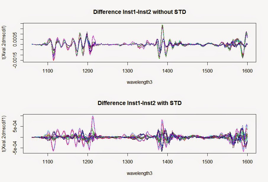
Spectra plots also will help us to understand how the STD correct the spectra, looking to the spectra and study the patterns we can see for wich samples works better or worse. We expect to see as much random noise as possible.

These plots are the validation samples of the Shootout 2002, with a standardization developed with a factor matrix multiplied to the unstandardized validation spectra. As said in previous posts, 8 samples were selected, but other samples could give (or not) similar plots.

Selection of samples is an important task. What is clear is that with the STD applied we get much better statistics as we saw in the post: "Standardizing the spectra (Shootout 2002)".

 

 

 

 

Plots to prepare the STD

In the previous post 8 samples were selected for the STD.

First figure shows the selected samples for the STD scanned (raw spectra) in Instrument 1 and 2, and the differences between them.

 

We can see the same procedure, but in this case the comparative is done with math-treatments (2º Derivative + MSC). As expected much more peaks in the spectra of the difference:

 

In a recent article from Mark Westerhaus to NIR News, he advice about the importance to check and review these plots and its shape, in order to apply the best standardization (single or multiple).

Comparing with more details the spectra, there are differences in the instruments not only in the photometric scale, also in the wavelength positions and in the bandwidth, but this differences are not constant all along the wavelength axis.

Actually manufacturers are improving the instruments to match each other, specially in the wavelength axis where more complex agorithms for correction are needed.

Some script with the Shootout 2002 data

This is some script to check ho it performs a model developed with the training set C1  using the other sets T1 and V1, and C2,T2 and V2. All the sets from instrument 2 need a bias adjustment in order to transfer the model from Instrument 1 (mod3a) to instrument 2.

library(pls)
#Quitamos las 5 muestras que se observan como anómalas
#en el conjunto de calibración C1, que coinciden con las
#anomalas del conjunto de calibración C2.
nir.tr1a.2dmsc<-nir.tr1.2dmsc[c(-19,-122,-126,-127,-150),]
#Quitamos las muestras anomalas también de la matriz Y
#Hacemos la regressión con C1
mod3a<-plsr(Y~X,data=nir.tr1a.2dmsc,ncomp=10,validation="LOO")

#############  Validando con Test1 sin 7 anómalos
test1a.pred<-as.matrix(predict(mod3a,ncomp=3,newdata=nir.test1.2dmsc))
monit.test1a<-cbind(Y.test,test1a.pred)   #para poder usar la función monitor
#Tenemos que dar nombres a las columnas y poner el mismo número de decimales
colnames(monit.test1a)<-c("Y.test.lab","Y.test.pred")
monit.test1a<-round(monit.test1a,digits=1)
monitor14(monit.test1a[,2],monit.test1a[,1],150,3,0.95,2.904)
#Al predecir el conjunto de Test1, en el modelo mod3a, observaremos si tenemos anómalos.
#Se observa las muestras anómalas entre la linea de Warning i action:
# Las muestras son: 5,9,145,294,313,341 y 342.
nir.test1a.2dmsc<-nir.test1.2dmsc[c(-5,-9,-145,-294,-313,-341,-342),]
test1a.pred<-as.matrix(predict(mod3a,ncomp=3,newdata=nir.test1a.2dmsc))
monit.test1a<-cbind(nir.test1a.2dmsc$Y,test1a.pred)     #para poder usar la función monitor
colnames(monit.test1a)<-c("Y.test.lab","Y.test.pred")
monit.test1a<-round(monit.test1a,digits=1)
monitor14(monit.test1a[,2],monit.test1a[,1],150,3,0.95,2.904)
##  RMSEP: 3.05

#############  Validando con Val1  ################################
val1a.pred<-as.matrix(predict(mod3,ncomp=3,newdata=nir.val1.2dmsc))
monit.val1a<-cbind(Y.val,val1a.pred)   #para poder usar la función monitor
colnames(monit.val1a)<-c("Y.val.lab","Y.val.pred")
monit.val1a<-round(monit.val1a,digits=1)
monitor14(monit.val1a[,2],monit.val1a[,1],150,3,0.95,2.904)
##  RMSEP    : 3.676

#############  Validando con C2  ######################################
#Quitamos las muestras anómalas del conjunto de calibración C2
nir.tr2a.2dmsc<-nir.tr2.2dmsc[c(-19,-122,-126,-127,-150),]
tr2a.pred<-as.matrix(predict(mod3a,ncomp=3,newdata=nir.tr2a.2dmsc))
#para poder usar la función monitor
monit.tr2a<-cbind(nir.tr2a.2dmsc$Y,tr2a.pred) 
#Tenemos que dar nombres a las columnas y poner el mismo número de decimales
colnames(monit.tr2a)<-c("Y.tr.lab","Y.tr2.pred")
monit.tr2a<-round(monit.tr2a,digits=1)
monitor14(monit.tr2a[,2],monit.tr2a[,1],150,3,0.95,2.904)
#  RMSEP: 3.642
#  Bias : -2.249
#  SEP  : 2.875
#***Bias adjustment is recommended***

#############  Validando con Test2 sin 7 anomalos  ##############
test2a.pred<-as.matrix(predict(mod3a,ncomp=3,newdata=nir.test2.2dmsc))
monit.test2a<-cbind(Y.test,test2a.pred)   #para poder usar la función monitor
#Tenemos que dar nombres a las columnas y poner el mismo número de decimales
colnames(monit.test2a)<-c("Y.test.lab","Y.test.pred")
monit.test2a<-round(monit.test2a,digits=1)
monitor14(monit.test2a[,2],monit.test2a[,1],150,3,0.95,2.904)
#Al predecir el conjunto de Test2, en el modelo mod3a, observaremos si tenemos anómalos.
#Se observa las muestras anómalas entre la linea de Warning y action:
# Las muestras son: 5,9,145,294,313,341 y 342.
nir.test2a.2dmsc<-nir.test2.2dmsc[c(-5,-9,-145,-294,-313,-341,-342),]
test2a.pred<-as.matrix(predict(mod3a,ncomp=3,newdata=nir.test2a.2dmsc))
monit.test2a<-cbind(nir.test2a.2dmsc$Y,test2a.pred)     #para poder usar la función monitor
colnames(monit.test2a)<-c("Y.test.lab","Y.test.pred")
monit.test2a<-round(monit.test2a,digits=1)
monitor14(monit.test2a[,2],monit.test2a[,1],150,3,0.95,2.904)
# RMSEP: 3.358
# Bias : -1.712
# SEP  : 2.892
#***Bias adjustment is recommended***

#############  Validando con Val2  #################################
val2a.pred<-as.matrix(predict(mod3,ncomp=3,newdata=nir.val2.2dmsc))
monit.val2a<-cbind(Y.val,val2a.pred)   #para poder usar la función monitor
colnames(monit.val2a)<-c("Y.val.lab","Y.val.pred")
monit.val2a<-round(monit.val2a,digits=1)
monitor14(monit.val2a[,2],monit.val1a[,1],150,3,0.95,2.904)
# RMSEP    : 5.635
# Bias     : -4.688
# SEP      : 3.168
#***Bias adjustment is recommended***

Recalculating the PLSR without outliers

When we developed the regression, we did nor remove any outliers from the calibration set, but now we are going to remove the 5 samples which seem clearly outliers, so we can give to results to the summary of the Shootout 2002, one will be the Standard Errors  of Prediction with all the samples, and other without these 5 samples (19,122,126,127 and 150).

These five samples are the same in the Training Set scanned in Instrument 1 and the Training Set scanned in Instrument 2, so it is clear that the problem is that the lab value does not correlate as the others with the spectra.

First, we remove the samples from the Training Set 1:

nir.tr1a.2dmsc<-nir.tr1.2dmsc[c(-19,-122,-126,-127,-150),]

Now, the new regression model without outliers, and with the math treatments we consider apropiate as MSC + Second derivative:

mod3a<-plsr(Y~X,data=nir.tr1a.2dmsc,ncomp=10,validation="LOO")

Comparing the summaries of the models with and without outliers we see the logical improvement.

 

We decide to use 3 terms in the model to predict the other sets. First we predict the Training Set scanned in Instrument 2, but without the 5 outliers:

nir.tr2a.2dmsc<-nir.tr2.2dmsc[c(-19,-122,-126,-127,-150),]

tr2a.pred<-as.matrix(predict(mod3a,ncomp=3,newdata=nir.tr2a.2dmsc))
monit.tr2a<-cbind(nir.tr2a.2dmsc$Y,tr2a.pred) 
monit.tr2 colnames(monit.tr2a)<-c("Y.tr.lab","Y.tr2.pred")
monit.tr2a<-round(monit.tr2a,digits=1)

Now with this table we can run the Monitor function:

monitor14(monit.tr2a[,2],monit.tr2a[,1],150,3,0.95,2.904)

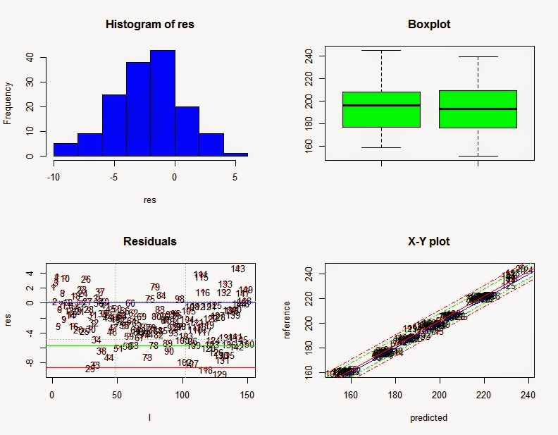
The results show an improvement in the RMSEP and the SEP statistic tell us the error corrected by the bias. The monitor function now recommend a Bias adjustment.

The distribution of the residuals shows the bias problem, but it is quite uniform once we correct the bias.

 

 

------------------------------------- 
N Validation Samples  = 150 
N Calibration Samples = 150 
N Calibration Terms   = 3 
------------------------------------- 
RMSEP    : 3.642 
Bias     : -2.249 
SEP      : 2.875 
UECLs    : 3.327 
***SEP is bellow BCLs (O.K)***
Corr     : 0.9917 
RSQ      : 0.9834 
Slope    : 1.002 
Intercept: 1.874 
RER      : 29.92   Good 
RPD      : 7.759   Very Good 
BCL(+/-): 0.4637 
***Bias adjustment is recommended***
Residual Std Dev is : 2.884 
***Slope adjustment in not necessary***

Monitor function 27-11-2014

Once developed a model with the math treatments we consider adequate, and using the Calibration Samples for Instrument 1 (following with the Shootout_2002 tutorial), the idea is to check if that model performs fine with Instrument 2 for exactly the same samples. A bias is expected, because even being the same model of instrument, differences in the hardware components, optics, alignments,…, apart from some others are the cause of this bias.

Some time ago I develop a function to monitor, to plot and obtain the statistics necessaries to take some decisions as if the bias or slope should be adjusted, to check for outliers of high residuals,.....

 

It is clear that we have 5 outliers of high residuals that the literature about this set considers that must be removed, so the error RMSEP will decrease.
Due to the high RMSEP of the model used for this monitor (RMSEP=4.33 using 4 terms and with all the samples), the bias must be quite high in order to be consider that it should be adjusted. This error is more than 3 times the Lab error.

So the statistics are:

monitor14(monit.tr2[,2],monit.tr2[,1],155,4,0.95,4.33)

Where 0.95 is the confidence interval and 4.33 the CV error of the model using 4 terms

N Validation Samples  = 155 
N Calibration Samples = 155 
N Calibration Terms   = 4 
------------------------------------- 
RMSEP    : 4.942 
Bias     : -2.509 
SEP      : 4.272 
UECLs    : 4.951 
***SEP is bellow BCLs (O.K)***
Corr     : 0.9811 
RSQ      : 0.9626 
Slope    : 0.9813 
Intercept: 6.122 
RER      : 19.9   Fair 
RPD      : 5.146   Good 
BCL(+/-): 0.6778 
***Bias adjustment in not necessary***
Residual Std Dev is : 4.266 
***Slope adjustment in not necessary***

We can see how the SEP (error corrected by the bias) is similar to the error of 

the model, so a bias adjustment will help to transfer the model from instrument 1

to Instrument 2.

I will remove the 5 samples and come back with the results.

SG 2nd Derivative + MSC

As you know derivatives remove the baseline offset and curvature in the spectra, but the should be combined with anti-scatter math treatments if we want to remove scatter effects which affect the correlation between the constituents of interest and the spectral bands. There are some cases (especially when developing discriminant models), where it is not convenient to apply the anti-scatter math treatments and we just leave the derivatives alone.

Following the Shoot-out tutorial and following the paper "Shoot-out 2002: transfer of calibration for content of active in a pharmaceutical tablet", from David W. Hopkins (NIR news Vol14 No. 5 2003), I tried the math treatment recommended by the author and apply the MSC after the SG2D1104, just to have a look to the spectra:

You can see how the red spectra, has been calculated in the previous post, and for the green one (SG second derivative combined with MSC), I use the following script:

> X1_sg2dmsc<-msc(X1_sg2d_pracma)
> matplot(wavelength2[11:281],t(X1_sg2dmsc[,11:281]),type="l",
+ xlab="Wavelength (nm)",ylab="1/R (SG 2nd der + MSC)",lty=1,
+ col=3,main="SG-2D1104 + MSC")
If we want to see them over-plotted

Applying SG to all our X matrix (Pracma Package)

"R" is without any doubt a great and wonderful community,  and it is nice to see how the package developers and maintainers help you in case you have any doubts.

It was the case some time ago when was writing some posts about the ChemoSpec package and Bryan Hanson helps me with some doubts. After the last post, I wrote a mail to Hans Werner (Pracma Package) , and he replied quickly, telling me the reason the "savgol" function use a vector indeed a matrix, and giving to me some ideas, to convert all the spectra matrix to Savitzky Golay.

Of course one of the ways is to use the apply function. When applying the SG filters there is  a reduction in the number of data-points at both sides of the wavelengths, depending of the window size.

 So I tried this way, to see all the spectra together:

> library(pracma)
# This script is for first derivative
> X1_sg1d_pracma<-apply(nir.training1$X,1,savgol,11,4,1)
> matplot(wavelength2[11:281],(X1_sg_pracma
+[11:281,]),type="l",xlab="Wavelength (nm)",
+ ylab="1/R (SG 1st derivative)",lty=1,col=1,main="SG-1D1104")

 

# This script is for second derivative
> X1_sg2d_pracma<-apply(nir.training1$X,1,savgol,11,4,2)
> matplot(wavelength2[11:281],(X1_sg_pracma
+[11:281,]),type="l",xlab="Wavelength (nm)",
+ ylab="1/R (SG 2nd derivative)",lty=1,col=1,main="SG-2D1104")

 

Savitzky Golay filters with Pracma Package

Pracma package has the function "savgol", where we can apply Savitzky Golay filter to a vector (in our case a spectrum).
The function is:
  savgol(T, fl, forder, dorder)

And the Arguments are:
 T... Vector of signals to be filtered.
fl... Filter length (for instance fl = 51..151), has to be odd.
forder... Filter order (2 = quadratic filter, 4 = quartic).
dorder... Derivative order (0 = smoothing, 1 = first der, etc.).

As you know I´m using in my last post the shoot-out 2002 data to develop a tutorial, and I read an article from the winner of this shoot-out where he use the shoot-out spectra with Savitzky Golay, a filter of 11, quartic, and second derivative using the Unscrambler software.

So I try thess values in the arguments of the Pracma SG filter and the results of the bands look exactly the same that the ones in the article, so this option looks good to work with this data. Anyway I will try also with the other functions from other packages.

In the case of the Pracma package we have to use a vector (a single spectrum), so some work has to be done to convert all the matrix of spectra, but the results looks great.

X1_sg_pracma<-as.matrix(savgol(nir.training1$X[1,],11,4,2))

PCAs with three diferent methods and projections (Test and Val Set)

The shoot-out 2012 is composed with 155 samples for the training set (Blue color), 460 for the Test Set (Red color), and other few samples for the Validation set (Green color).

I have developed 3 different ways of Principal Components Analysis and I would like to show you the score plot of PC1 vs PC2 developed with the Training Set and the projections on that space of the Test and Validation Set.

This first plot is in the case  of using PRCOMP:

Second case is using NIPALS for the calculation of the PCAs:

and third using SVD for the calculation of the PCAs

As you can see no differences, and we can have the conclussions that the Training Set cover the variability for the samples of the Test Set and Validation Set, so we don´t have to extrapolate outside the calibration space.

I will writte a post with the code (quite long) if interested. Let me know.

 

Adding Category Variables to a Data frame in R

Normally I used data frames to manage NIR data, the data frames are composed normally in my case by a X  or Spectra matrix (dataframe$X), and a Y or constituent matrix (dataframe$Y). But when we want to manage and understand plots, like score plots, it is interesting to classify the samples with some category variables.

This category variables can be: "location", "type", "customer", "product",.....

In the case of the shoot-out data the samples can be classify by their content of the main parameter, and can be classified as:

"Low"             (if the sample has less than 160 mg)
"Medium"          (between 160 y 221 mg)
"High"            (more than 221 mg)

Let´s create the variable in the data frame of the training set for instrument 1
nir.training1$type[Y <=160] <- "Low"
nir.training1$type[Y>160 & Y<221] <- "Medium"
nir.training1$type[Y>=221] <- "High"
Now we have a new variable in the data frame called "type"
Check it with:

names(dataframe)

and appart from X and Y we have Type.

We proceed the same way for the other dataframes.

Another thing is that we can create a big data frame with all the spectra from different instruments and sets and create a category variable for the instrument ( A and B), and another for the Set (Training, Test and Validation).

SNV + Detrend with "Prospectr" package

I was using the function “detrend” from the “pracma” package, but we have the detrend function in the “prospectr” package. Using this last option we combine the SNV with the Detrend, which is a very common math-treatment to remove the scatter.

Looking to the function script the “sweep” function is used to center and scale the spectra matrix.

 

Using the shootout 2002 data:

>X1_detrend2<-detrend(nir.training1$X,

+wav=as.numeric(colnames(nir.training1$X)))

>matplot(wavelength2,t(X1_detrend2),type="l",lty=1,

+xlab="Wavelength(nm)",ylab="1/R",col=3,

+main="SNV + Detrend")

I compare with these plots the way prospectr runs the SNV detrend versus the other way I used in other posts.

Green with prospectr package and blue with pracma package.

2nd derivative using "apply" and "diff"

This is a simply exercise, where we convert the raw spectrum into its first derivative, and into its second derivative, using the function apply, and the function diff.

I use the shootout 2002 data available in the package ChemometricsWithR.

X1_diff1<-t(apply(nir.training1$X,1,diff))

In this case the 1 is to apply the function difference to the rows (spectra).

We don´t add more than the default options to the function diff, so the lag=1 and the value of differences=1.

The spectrum changes (losing 1 data point) to the black spectrum in the plot at the end of the post.

plot(as.numeric(colnames(X1_diff1)),X1_diff1 [1,],type="l",xlab="Wavelength (nm)",ylab="1/R (1st derivative)",lty=1,col=1)

We can say briefly that the second derivative is the derivative of the firs derivative; we can do this changing the value of the option “differences” from 1 to 2, losing, in this case two data points.

X1_diff2<-t(apply(nir.training1$X,1,diff,differences=2))

par(new=TRUE)

plot(as.numeric(colnames(X1_diff2)),X1_diff2[1,],type="l",xlab="Wavelength (nm)",ylab="1/R (2nd derivative)",lty=1,col=2)

The spectrum of the second derivative is the red one in the plot, compared with the black one of the first derivative.

This way to do the derivatives is very noisy, so in future post we will try to use gap derivative which is the way that softwares as Unscrambler, Win ISI and many others use the derivatives.

Comparing regressions with different scatter math-treatments (Shootout 2002 Tutorial)

In a previous post, we have developed the calibration without any math-treatment with the Training Set from Instrument 1, without any treatment , knowing that it was not the best choice, and we look to the LOO (leave one out) cross validation errors to check the performance.

Now we develop the regressions with some anti-scatter math-treatments to compare the cross validation errors and to decide which of them performs better. Anyway the shootout supplies also a test set, so validating with this test set will give us a better idea about how the calibration is performing with independent data.

 

First thing to do is to convert the “X1. Training” and “X1. Test” matrix to the math treatment we want to use: SNV (Standard Normal Variate), Detrend , SNV + Detrend and MSC.

>nir.train1_snv<-data.frame(X= I(X1_snv),Y=I(Y))

>nir.train1_detrend<-data.frame(X= I(t(X1_detrend)),Y=I(Y))

>nir.train1_snvdt<-data.frame(X= I(t(X1_snvdt)),Y=I(Y))

>nir.train1_msc<-data.frame(X= I(X1_msc),Y=I(Y))

Now we can develop the PLS regressions:

 

>mod1_snv<-plsr(Y~X,data=nir.train1_snv,+

 ncomp=10,validation="LOO")

>mod1_detrend<-plsr (Y~X,data=nir.train1_detrend,+

 ncomp=10,validation="LOO")

>mod1_snvdt<-plsr(Y~X,data=nir.train1_snvdt,+

 ncomp=10,validation="LOO")

>mod1_msc<-plsr(Y~X,data=nir.train1_msc,+

 ncomp=10,validation="LOO")

We can plot the RMSEP values versus the number of components (or terms), to have a better idea of the performance of the models (black line is the model without mat-treatments or raw spectra, green line is with just Detrend, the rest (SNV, SNV+DT and MSC) are almost overlaped.

 

But if we want to see it with more details, we have to see the numbers provided by the summary of the models. I mark in yellow the smallest values.

 

 

But the question can be: Do we have to choose the number of components which gives the small RMSEP?.

We will reply to this question soon.

In a next post we will do the same with derivative mixed with scatter corrections to see if we get better values for RMSEP and we will check it with an external validation (don´t forget that these RMSEP are for Cross Validation).

 

 

 

 

 

 

SNV and Detrend (Shootout 2002 NIR with R)

I want to say “thanks” to Aoife Gowen (@eefieg) for the references, in her last article to this blog. The article is the part 4 of a series called “NIR hyperspectral image analysis using R” and the title of this article is: "Pretreatments and partial least square discriminant analysis". (NIR News Vol.25 Nº 5 August 2014).
 

Lately I am playing with the Shootout 2002 data so we can summarize on this data things that we have seen before in the blog.
 

In the last post, I was using the raw spectra and that is not (in some cases) the best way to develop a calibration. So we treat the raw spectra with math treatments to improve the correlation of the spectra with the reference values, and to make more transferable calibrations. If we use a correct math-treatment the regressions will use less terms, and will improve the statistics, and the transferability.

Now I write the script used to treat the matrix X1 (training spectra matrix in Instrument 1):

>par(mfrow=c(2,2),ps=14)
>matplot(indices,t(nir.training1$X),type="l",col=1,

 + main="Raw Spectra")
#Applying "SNV" to the Shootout 2012 Data>X1_snv<-scale(t(nir.training1$X),center=TRUE,scale=TRUE)
>matplot(wavelength2,X1_snv,type="l",

 + xlab="Wavelength (nm)",ylab="1/R",lty=1,

 + col=2,main="SNV math_treat")
#Applying "Detrend" to the Shootout 2012 Data

>library(pracma)
>X1_detrend<-detrend(t(nir.training1$X))  
 +matplot(wavelength2,X1_detrend,type="l",

 +lty=1,xlab="Wavelength(nm)",ylab="1/R",col=3,

 +main="Detrend math_treat")
#Combining SNV with Detrend

>X1_snvdt<-detrend(X1_snv,tt="linear")

>matplot(wavelength2,X1_snvdt,type="l",lty=1,

 +xlab="Wavelength(nm)",ylab="1/R",col=4,

 +main=" SNV+Detrend math-treat")

 

As we are writing this script, we see on the Active Graphics Window the spectra , so we can compare them.

These are some of the most familiar anti-scatter math-treatments, apart from others like MSC.

 

We will continue with this type of exercises in the next posts.

XY Plot to compare predictions (same model / diferent instruments)

As we mention several times, plots help us to understand better what is happening. In the previous posts we are working with the shootout 2002 data in order to work with as many tools as possible we have in R to understand this data set and to make a model we can use to predict as better as possible a validation set.
Plotting the predictions of the Test set acquired in Instrument 2 with the model developed with the Training set of samples acquired in Instrument 1, versus the predictions of the test set acquired in instrument 1, can give us an idea that there is something more than a simple bias, and that we have to take into account a group of samples that behaves differently.
Lets see that plot:
1) We make the predictions of the Test1 set with Model 1 and stored it in:
  anl_tst1_mod1<-predict(mod1,ncomp=3,
+ newdata=data.frame(Y=I(Y.test),X=I(X1.test)))
2) We make the predictions of the Test2 set with Model 1 and stored it in:
  anl_tst2_mod1<-predict(mod1,ncomp=3,
+ newdata=data.frame(Y=I(Y.test),X=I(X2.test)))
3) Now we plot the predictions versus reference for anl_tst1_mod1
  plot(Y.test,anl_tst1_mod1,col="blue",ylim=c(150,240))
4) Now we write the script:
   par(new=TRUE)
5) Now we plot the predictions versus reference for anl_tst2_mod1
  plot(Y.test,anl_tst2_mod1,col="red",ylim=c(150,240))
6) Now we get this plot:

We can see that most of the samples behave similarly with a bias

 

If interested to follow this tutorial see also:

Working with the Shootout 2002 (NIR) in R

Plotting the predictions (Working with the Shootout 2012 NIR data in R)

Comparing Spectra and Coefficients (Shootout 2002 NIR with R)

 

 

 

Comparing Spectra and Coefficients (Shootout 2002 NIR with R)

We can check the differences between the instruments 1 and 2 more in different ways. One could be to select 5 samples, and compare their spectra scanned in Instrument 1 and scanned in instrument 2. In this case I select from the training set samples 10,20,30,40 and 50.
The samples look like this:

But the best to see the differences, is to substract the spectra, so I made some substractions:
dif1<-selected[1,]-selected[6,]
dif2<-selected[2,]-selected[7,]
dif3<-selected[3,]-selected[8,]
dif4<-selected[4,]-selected[9,]
dif5<-selected[5,]-selected[10,]
and combined them:
dif<-rbind(dif1,dif2,dif3,dif4,dif5)
Now we can see the spectra of the differences (quite similar for the 5):

 

 

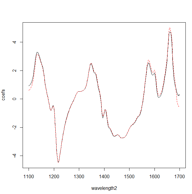
When developing the models (mod 1 and mod 2), we obtain the regression coefficient, which are like a spectra, so we can compare them:

 

 

and also substract them:

 

to obtain some conclussions.

 

 

 

 

 

Plotting the predictions (Working with the Shootout 2012 NIR data in R)

This post follows the previous one: "Working with the Shootout 2012 (NIR) in R".
We have predicted the Test file scanned in Instrument 2 with the model developed with the Training file scanned in Instrument 1 (mod 1), and we have seen that the RMSEP is higher than the RMSEP obtained predicting the Test file scanned in Instrument 1 with the same model mod1. The X-Y plot will give us a better idea of what is going on.
This figure represents the predictions of the Test Set scanned in instrument 1 with the model mod1:
predplot(mod1,ncomp=3,newdata=data.frame(Y=I(Y.test),X=I(X1.test)),
asp=1,line=TRUE)

The next figure represents the predictions of the Test Set scanned in instrument 2 with the model mod1:

predplot(mod1,ncomp=3,newdata=data.frame(Y=I(Y.test),X=I(X2.test)),

asp=1,line=TRUE)

We can see that part of the RMSEP error is due to an important bias, and an increase of the random noise.

This shootout is probably the most famous so there is quite enough articles and documents and as far as we continue with this tutorial, we can see the results compared with other approaches.

 

 

Working with the Shootout 2002 (NIR) in R

I was practicing with the shootout 2002, where you have a certain number of training samples (155), scanned in two instruments 1 and 2, so we have two "Training files" with the same LAB values, but different spectra (due that the samples are acquired in diferent instruments). The idea of the shootout is to develop a robust calibration for both instruments.

So I had  developed a PLS Model in R with the Training samples acquired in "Instrument 1". I called the model "mod1":

mod1<-plsr(Y~X1,data=nir.training1,ncomp=5,validation="LOO").

Where "nir.training1" is a data frame:

nir.training1<-data.frame(X= I(X1),Y=I(Y))

X: is the 155 row training matrix of spectra acquired in Instrument 1

Y: is the reference training matrix of the constituent of interest and this matrix is the same for the Instrument 2, where their matrix of spectra would be X2.

 

after checking the summary of the model I decide that 3 terms (components) are enough for the model.

 

Now  I want to predict the samples of  a Test file (also scanned in 1). This Test file has more samples  (460), so the rows are higher for the Y matrix and for the X matrix. The idea is to get a RMSEP statistic.

RMSEP(mod1,estimate="test",ncomp=3,intercept=FALSE,

+ newdata=data.frame(Y=I(Y.test),X=I(X1.test)))

 

 and I have found several problems getting errors like this:

"newdata' had 460 rows but variables found have 155 rows"

"Error en model.frame.default(formula(object), data = newdata) :

variable lengths differ (found for 'X1')".

I was making some mistakes assigning names to the matrix in the data frame, and they must be the same in both cases (The dataframe from which I develop the regression and the dataframe which I want to evaluate.

nir.training1<-data.frame(X= I(X1),Y=I(Y))

newdata=data.frame(Y=I(Y.test),X=I(X1.test)))

 

Finally I got a value of 4.974 for the RMSEP.

Now the following exercise must be to check if I have a similar error with a calibration develop with a model developed with the Training spectra of Instrument 2 with the Test Set spectra from Instrument 2 (don´t forget that the Y reference values are the same that for instrument 1, because we are using the same samples):
mod2<-plsr(Y~X,data=nir.training2,ncomp=5,validation="LOO")
Three terms are also enough, and the RMSEP for the Test Set scanned in Instrument 2 with the model 2 is:
RMSEP(mod2,estimate="test",ncomp=3,intercept=FALSE,
+ newdata=data.frame(Y=I(Y.test),X=I(X2.test)))

 and the value is: 5,315.

But what would be the RMSEP for the Test set scanned in Instrument 2 and predicted with the model developed with the Training Samples scanned in instriment 1 (mod1):
RMSEP(mod1,estimate="test",ncomp=3,intercept=FALSE,
+ newdata=data.frame(Y=I(Y.test),X=I(X2.test)))

 The result is: 9,983
So the model can not be transfered without doing anything from instrument 1 to Instrument 2, if what we want is to get similar performance in both.
We will continue with this in the next post.