Tratamientos anti-scatter con R-Notebooks

Scatter Correction Spectra plots with R

These are the spectra of an Infratec 1241 for Soy meal treated with "Multiple Scatter Correction", "Standard Normal Variate" and "Standard Normal Variate  + Detrend", apart from the "Raw Spectra".

All this math treatments are in the new Video Series (in spanish) from the posts last weeks.

In next post we see the effect of derivatives in the spectra, and we continue with Principal Components and Regressions Methods.

Detrend (grade 2) calculation in Excel

In the previous post we calculate the  detrend math treatment with the linear option, but normally the detrend has a curvature caused by the scatter so we have to calculate the correction with a quadratic equation and subtract every data point of that curve from the raw spectra to get the corrected spectra.

Detrend (grade 1) calculation in Excel

Just represent a spectrum in Excel, and calculate a linear regression (slope and intercept). Calculate the values of that line and subtract them from the spectra, ...., you will get a Detrend Correction of Grade 1 (linear and offset).

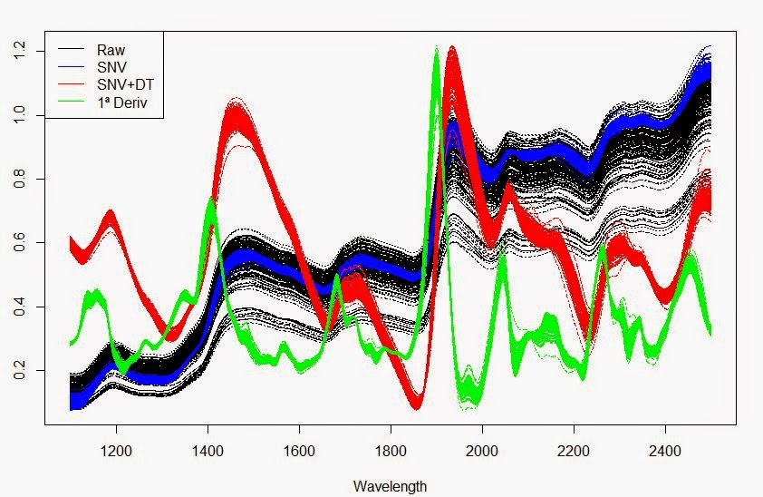
Some script using "prospectr"

library(prospectr)
hsoja.X<-as.matrix(read.table("clipboard",header=FALSE))
wavelength1<-seq(from=1100.0,to=2499.5, by=0.5)
X.ID<-seq(from=1,to=159, by=1)
colnames(hsoja.X)<-wavelength1
rownames(hsoja.X)<-X.ID
plot(as.numeric(colnames(hsoja.X)),hsoja.X[1,],
   +type="l",xlab="wavelength",ylab="Absorbance")
matplot(wavelength1,t(hsoja.X),type="l")
hsoja.X.bin<-binning(hsoja.X,bin.size=4)
wavelength2<-seq(from=1100,to=2498, by=2)
colnames(hsoja.X.bin)<-wavelength2
matplot(wavelength2,t(hsoja.X.bin),type="l",
ylab="",xlab="Wavelength")
points(as.numeric(colnames(hsoja.X.bin)),
   +hsoja.X.bin[1,],pch=2)
matplot(wavelength1,t(hsoja.X),type="l",ylab="",
   +xlab="Wavelength",col="black")
par(new=T)
hsoja.Xsnv<-standardNormalVariate(X=hsoja.X)
matplot(wavelength1,t(hsoja.Xsnv),type="l",xaxt="n",
   +yaxt="n",ylab="",xlab="",col="blue")
hsoja.Xsnvdt<-detrend(X=hsoja.X,wav=as.numeric(colnames(hsoja.X)))
par(new=T)
matplot(wavelength1,t(hsoja.Xsnvdt),type="l",
xaxt="n",yaxt="n",xlab="",ylab="",col="red")
h.soja.snvdt1d<-t(diff(t(hsoja.Xsnvdt),differences=1,lag=16))
wavelength3<-seq(from=1108,to=2499.5, by=0.5)
par(new=T)
matplot(wavelength3,t(h.soja.snvdt1d),type="l",
   +xaxt="n",yaxt="n",xlab="",ylab="",col="green")
# All the sequence for the plot
matplot(wavelength1,t(hsoja.X),type="l",
   +ylab="",xlab="Wavelength",col="black")
par(new=T)
matplot(wavelength1,t(hsoja.Xsnv),type="l",
   +xaxt="n",yaxt="n",ylab="",xlab="",col=4)
par(new=T)
matplot(wavelength1,t(hsoja.Xsnvdt),type="l",
   +xaxt="n",yaxt="n",xlab="",ylab="",col=2)
par(new=T)
matplot(wavelength3,t(h.soja.snvdt1d),
   +type="l",xaxt="n",yaxt="n",xlab="",ylab="",col="green")
legend("topleft",legend=c("Raw","SNV","SNV+DT","1ª Deriv"),
   +lty=c(1,1),col=c("black","blue","red","green"))

SG 2nd Derivative + MSC

As you know derivatives remove the baseline offset and curvature in the spectra, but the should be combined with anti-scatter math treatments if we want to remove scatter effects which affect the correlation between the constituents of interest and the spectral bands. There are some cases (especially when developing discriminant models), where it is not convenient to apply the anti-scatter math treatments and we just leave the derivatives alone.

Following the Shoot-out tutorial and following the paper "Shoot-out 2002: transfer of calibration for content of active in a pharmaceutical tablet", from David W. Hopkins (NIR news Vol14 No. 5 2003), I tried the math treatment recommended by the author and apply the MSC after the SG2D1104, just to have a look to the spectra:

You can see how the red spectra, has been calculated in the previous post, and for the green one (SG second derivative combined with MSC), I use the following script:

> X1_sg2dmsc<-msc(X1_sg2d_pracma)
> matplot(wavelength2[11:281],t(X1_sg2dmsc[,11:281]),type="l",
+ xlab="Wavelength (nm)",ylab="1/R (SG 2nd der + MSC)",lty=1,
+ col=3,main="SG-2D1104 + MSC")
If we want to see them over-plotted

SNV + Detrend with "Prospectr" package

I was using the function “detrend” from the “pracma” package, but we have the detrend function in the “prospectr” package. Using this last option we combine the SNV with the Detrend, which is a very common math-treatment to remove the scatter.

Looking to the function script the “sweep” function is used to center and scale the spectra matrix.

 

Using the shootout 2002 data:

>X1_detrend2<-detrend(nir.training1$X,

+wav=as.numeric(colnames(nir.training1$X)))

>matplot(wavelength2,t(X1_detrend2),type="l",lty=1,

+xlab="Wavelength(nm)",ylab="1/R",col=3,

+main="SNV + Detrend")

I compare with these plots the way prospectr runs the SNV detrend versus the other way I used in other posts.

Green with prospectr package and blue with pracma package.

Applying "Detrend" to the spectra with R

There is a nice math treatment I use to apply to the spectra in NIR. It is the Detrend.
Normally goes together with the SNV, but this time I´m going to apply it alone.
I´m going to use the Yarn data, with this raw spectra:

 

 

Now we load the R package "pracma":

 

library(pracma)

yarndt_NIR<-detrend(t(yarn$NIR),tt="linear")

wavelengths1<-seq(1,268,by=1)  #para "yarn"

matplot(wavelengths1,yarndt_NIR,type="l",lty=1,

+xlab="Wavelength(nm)",ylab="1/R")

 

The spectra change to this one:

 

We can see hou the "trend" effect ( a shift in the baseline) is corrected and the baseline adjusted.

:

Polynomial trendline - Excel

El llamado “scatter” en los espectros NIR, hace que la línea de base se desvíe a medida que aumenta la longitud de onda. Con el fin de corregir esta desviación nos hemos referido anteriormente al tratamiento matemático “Detrend” el cual aplica un polinomio de 2º grado para después restarlo a cada valor de absorción en cada longitud de onda.

Excel nos permite trazar la línea de ese polinomio sobre el espectro, con la opción: Format Trendline.
 

“Scatter makes that the baseline shifts upwards in NIR spectrum as the wavelength increase. In order to reduce this effect we have talked in previous inputs about the mathematical treatment “Detrend”, which apply a 2 degree polynomial, in order to subtract it from the spectrum and correct the baseline.

Excel has a fuction where we can draw this polynomial over the spectrum with the Excel function: “Format Trendline”.
 

Detrend (2)

Los polinomios usados para el calculo del tratamamiento Detrend pueden ser de orden 0, 1 y 2. El software Vision nos permite seleccionar el orden, como podemos ver en el menu adjunto:

Estos tratamientos cambian el espectro  en la forma que hemos visto en la entrada anterior Detrend (1).
Información de como utiliza estos tratamientos Win ISI en "Learning Win ISI": Detrend en Win ISI.

Detrend (1)

El Detrend es un tratamiento para quitar los efectos de "offset" en la linea de base,ásí como la pendiente o curvatura de los espectros, normalmente causados por el "scatter", empaquetamiento,.... Se trata de un polinomio cuadrático.
El cálculo de esta función se resta del espectro original, dando como resultado el espectro con tratamiento detrend aplicado.
Normalmente se aplica conjuntamente a otros tratamientos (por lo general el SNV).
En la gráfica vemos los espectros sin tratamiento (negro), aplicando el orden "0" (azul) en el que quitamos el efecto del offset, aplicando el orden "1" (naranja) en el que quitamos el offset y la pendiente, y el de orden "2" (rojo) en el que quitamos los efectos de offset, pendiente y curvatura.
Ciertos softwares te permiten elegir el orden del polinomio.

Standar Normal Variate (SNV)

Otro tratamiento para corregir el scatter es el SNV. Se trata también de un autoescalado en el que a diferencia del MSC, interviene cada espectro de manera individual.

Para cada espectro, calculamos la media de todos los valores de absorción y también su desviación estándar. Restamos a cada "data point" el valor medio y el resultado lo dividimos por la desviación estándar. Este proceso se repite para cada uno de los "data poits" del espectro. Como resultado tendremos un nuevo espectro, con una varianza de uno. El proceso se repite para todos los espectros.

 

El espectro azul es el espectro sin tratamiento alguno y el rojo, es el mismo espectro con un tratamiento SNV.
Las características físicas de la muestra, intervienen en la escala espectral. En el caso de que queramos que no sean consideradas, un tratamiento anti-scatter es esencial para el desarrollo de la calibración. Sin embargo en el caso de los análisis discriminantes, el añadir este tipo de tratamientos debe de ser considerado.

Multiple Scatter Correction (MSC)

Leyendo un interesante artículo de T. Davies y T. Fearn sobre el tratamiento MSC en la revista Spectroscopy Europe, me puse a desarrollar uno de los gráficos que proponen para un mejor entendimiento de este tratamiento para la corrección del "scatter".
Para ello use los espectros del Shootout 2002, los exporté a Excel y calculé el espectro medio. Posteriormente en Excel representé el X-Y plot de la 1ª muestra del producto Calibra1, respecto al espectro medio de este mismo producto, obteniendo la siguiente gráfica:
Reading an interesting article by T. Davies & T. Fearn about MSC treatment in the journal Spectroscopy Europe, I began to develop one of the graphics proposed for a better understanding of this treatment for the correction of "scatter".
To do this use the spectra of the Shootout 2002, export to Excel and calculated the average spectrum. Later in Excel I represented the X-Y plot of the 1st sample of the product Calibra1, compared to the average spectrum of the same product, obtaining the following graph:

En esta gráfica, podemos calcular por mínimos cuadrados la pendiente y el intercepto que usaremos para corregir el scatter en este espectro en particular, pero haremos lo mismo con todos los espectros, respecto al espectro medio.
Para corregir el espectro, restaremos al valor de log1/T para cada data point el intercepto y dividiremos el resultado por la pendiente: (Xi - a)/b.
Debido a que este tratamiento se basa en el espectro medio del conjunto de datos original, si este se amplia este se debe de calcular nuevamente el espectro medio, así como la pendiente (b) e intercepto (a) de nuevo para cada espectro respecto al nuevo espectro medio, lo que representa un cierto inconveniente hasta que la base de datos sea lo suficientemente representativa.

In this graph, we can calculate least-squares slope and intercept that we will use to correct the scatter in this spectrum in particular, but will do the same with all spectra, compared to the average spectrum.
To correct a spectrum, subtract the value of log1 / T for each data point intercept and divide the result by the slope (Xi - a) / b.
Because this treatment is based on the average spectrum of the original data set, if we add more samples we should recalculate the average spectrum, the slope (b) and Intercept (a) again for each spectrum with respect to new media spectrum, representing some inconvenience until the database is sufficiently representative.

Conjunto Espectral sin ningun tratamiento:

(raw spectra)

Aplicando el tratamiento MSC:

(spectra corrected with MSC)