Comparing "R-PLS", "CARET" and "WIN ISI"

I made this exercise just for fun. When we develop a regression we don´t have to look the the XY plot where a sample is predicted from a model where this sample is already included, we have to compare it against a model where she is excluded. So we have to look to see how the samples fits to the regression line to the XY plot of Cross Validation for the number of terms we have selected for the final model.

 

In this case I develop the comparison for a regression of protein in fish meal with the 40 samples I am using in the series of tutorials about "Tidyverse and Chemometrics" using the PLS  and Caret packages and also Win ISI (FOSS Analytical Chemometric software).

 

PLS, Win ISI and Caret recommend 8 terms and as you can see they gave the same LOO Cross Validation XY plots or very similar. Remember that these are the XY plots of predictions where every sample is predicted with the 39 remaining so it´s more realistic of how it will performs in routine.

 

 

Linear Regressions to calculate the Loadings

We saw in previous post how the scores are calculated for every PLS term once we have the weights, so we start by t1 (scores on the first PLS term), and after we calculate the Loadings as regressions of X on T, so the loadings are spectra with values of "b" coefficients indeed absorbance. So they give us an idea of the importance of every wavelength in the term.

 

Every spectrum has 100 wavelength (850 to 1048 every 2 nm) so 850 is in the data point 1, 852 in the data point 2,........and 1048 in the data point 100.

 

So, we can make linear regressions on the X matrix (with its math treatment applied) on the score t1 calculated to get the value of every data point in the first loading.

 

The way to do it is:

lm(X_msc_centered[odd,10]~t1_pls)     #b=-1.247e-01
lm(X_msc_centered[odd,50]~t1_pls)     #b=-6.269e-02
lm(X_msc_centered[odd,90]~t1_pls)     #b= 1.348e-01

We can check after how this values are the same as the calculated for the PLS algorithm.

What condition must have the "loadings" in PLSR?

In the case of the loadings for PLS we do not have the condition of orthogonality as in the weights or scores, even if they are coming from orthogonal scores.

So the product of the matrices P^t.P is not a diagonal matrix, and this condition is what makes PLS regression special and different from Principal Components Regression.

Let´s check:
Xodd_pls3_ld1
Xodd_pls3_ld2
Xodd_pls3_ld3
Xodd_pls3_ld4
p.matrix<-cbind(Xodd_pls3_ld1,Xodd_pls3_ld2,
                Xodd_pls3_ld3,Xodd_pls3_ld4)

 > round(t(p.matrix) %*% p.matrix,4)
              Xodd_pls3_ld1 Xodd_pls3_ld2 Xodd_pls3_ld3 Xodd_pls3_ld4
Xodd_pls3_ld1        1.0132       -0.1151        0.0000        0.0000
Xodd_pls3_ld2       -0.1151        1.2019       -0.4493        0.0000
Xodd_pls3_ld3        0.0000       -0.4493        1.8783       -0.9372
Xodd_pls3_ld4        0.0000        0.0000       -0.9372        1.0134

We can see the red numbers that makes that we don´t get the condition of orthogonality, and how the loadings 2 and 3 are specially involved, and these is because in this case the loadings 1 and 4 are very similar to the weights 1 and 4, and 2 and 3 are quite different.

So loadings 1 and 4 are orthogonal between them. So there is no condition for the loadings.

What condition must have the scores in PLSR?

We have seen that the weights are orthogonal in PLSR regression (What condition must have the weights in PLSR?), so the scores, which are projections of the spectra over the weights must be orthogonal as well.

Let´s do the same operations than "What condition must have the weights in PLSR?":

Xodd_pls3$scores[,1]
Xodd_pls3$scores[,2]
Xodd_pls3$scores[,3]
Xodd_pls3$scores[,4]
t.matrix<-cbind(Xodd_pls3$scores[,1],Xodd_pls3$scores[,2],
                Xodd_pls3$scores[,3],Xodd_pls3$scores[,4])
round(t(t.matrix) %*% t.matrix,4)

         [,1]   [,2]   [,3]   [,4]
[1,] 146.3176 0.0000 0.0000 0.0000
[2,]   0.0000 0.4371 0.0000 0.0000
[3,]   0.0000 0.0000 0.0634 0.0000
[4,]   0.0000 0.0000 0.0000 0.0639

 

As we see we obtain a diagonal matrix, so the condition of orthogonality is fine.
But the difference with the weights, is that the weights, apart from being orthogonal, are  orthonormal, because are normalized to length one.

> round(t(w.matrix) %*% w.matrix,4)

Xodd_pls3_w1 Xodd_pls3_w2 Xodd_pls3_w3 Xodd_pls3_w4 Xodd_pls3_w1 1 0 0 0 Xodd_pls3_w2 0 1 0 0 Xodd_pls3_w3 0 0 1 0 Xodd_pls3_w4 0 0 0 1

 

What condition must have the weights in PLSR?

Well, this can be an easy question: "they are orthogonal between them", anyway I just want to check it, and the simple way is to combine all the weights in a matrix, and to multiply:

(Weight.matrix transposed)  * Weight.matrix

and the result must be the Identity Matrix. So let´s check it:
Xodd_pls3_w1
Xodd_pls3_w2
Xodd_pls3_w3
Xodd_pls3_w4
w.matrix<-cbind(Xodd_pls3_w1,Xodd_pls3_w2,
                Xodd_pls3_w3,Xodd_pls3_w4)
round(t(w.matrix) %*% w.matrix,4)

> round(t(w.matrix) %*% w.matrix,4)

            Xodd_pls3_w1 Xodd_pls3_w2 Xodd_pls3_w3 Xodd_pls3_w4 Xodd_pls3_w1   1 0     0 0 Xodd_pls3_w2   0 1     0 0 Xodd_pls3_w3   0 0     1 0 Xodd_pls3_w4   0 0     0          1

 
So the condition of orthogonality  is fine.

Understanding PLS Regression in a diagram

This is a first part of the diagram of how some of the inside parts of the algorithms works. the diagram still needs to grow with new steps adding new terms (this is just for the first term), and with the matrices "F" and "q".

 

The idea is to link all these diagrams to the Win ISI diagram.

 

Everything start with my previous posts:

How the Weights are calculated in PLS?
How the scores are calculated in PLS ?
How the loadings are calculated in PLS?

How the Weights are calculated in PLS

We have seen how the scores and loadings are calculated when developing a PLS regression, but what about the Weights?.

 

To calculate the X scores and the loadings we need the weights, and in particular the first one (to start all the process), after this calculation the scores are calculated as projections of the spectra on the weights, and after the scores are calculated we calculate the loadings.

The first weight is calculated a the Singular Value Decomposition of the cross product of X centered and transposed and Y, beeing X the spectra matrix and Y the constituent matrix.

When we do this we get (as we saw in other posts): "u", "d" and "v".

The first weight are the values in "u".

Xt<-t(X_msc_centered[odd,])  #100.327
Y<-as.matrix(Prot[odd,])     #327.1
Xt.Y<-Xt%*%Y                 #100.1
svd.XtY<-svd(Xt.Y)
dim(svd.XtY$d)
dim(svd.XtY$u) #100.1
plot(svd.XtY$u)
par(new=TRUE)
plot(Xodd_pls3_w1,type="l",col="red",lwd=2)

We continue in next post with the reconstruction of all the PLS process.

How the loadings are calculated in PLS?

After seeing "How the scores are calculated in the PLS" (in particular the scores for the first term), now I follow with "How the loadings are calculated in the PLS?" (and in particular the first loading.

Loadings are calculated as regressions of T on every column of X, so in this case we regress "t1_pls" (calculated on "How the scores are calculated in the PLS?") on X, and we do it in a matrix way and we scale it dividing by t(t1_pls)*t1_pls which is an scalar.

Xt.t1_pls<-t(X_msc_centered[odd,]) %*% t1_pls          
tt.t<-as.numeric(t(t1_pls)%*%t1_pls)
p1_pls<-Xt.t1_pls/tt.t

Now we can plot the reconstructed one with this code and the first loading we get from the "plsr" function of the pls package.

matplot(wavelengths,p1_pls,lty=1,pch=NULL,type="l",lwd=2,
        col="red",xlab="Wavelengths",ylab="Loadings Int.",
        ylim=c(-0.3,0.3))
par(new=TRUE)
matplot(wavelengths,Xodd_pls3_ld1,lty=2,pch=NULL,lwd=2,
        type="l",col="blue",xlab="",ylab="",
        ylim=c(-0.3,0.3))

and:
p1_pls==Xodd_pls3$loadings[,1]
we get TRUE for all the values.

How the scores are calculated in PLS

The first step in the PLS Regression is to calculate the weights, and as we said, there is one weight for every term of the regression, and we get them in the pls argument $weights, so in the case of the regression of the previous post the first weight is:

Xodd_pls3_w1<-as.matrix(Xodd_pls3$loading.weights[,1])
Now we have to project our samples spectra over this first weight to get the scores that we store in a vector "t_1", and with all the vectors (t_1, t_2,...., t_a) we will get the "T" matrix of pls scores.

To project the samples is a matrix multiplication:

 t_1= X.w1

Where X is the spectra matrix treated with MSC and centered and w1 is the first weight. 

As you know, to multiply matrices the number of columns of the first matrix must be the same as the number of rows of the second matrix.
So let´s check if our calculated values are the same as the PLS regression scores for the first PLS term:

dim(Xodd_pls3_w1)               #100*1
X_msc_centered<-scale(X_msc,
                      center=colMeans(X_msc[odd,])
                      ,scale=FALSE)
dim(X_msc_centered[odd,])       #327*100
t1_pls<-X_msc_centered[odd,] %*% Xodd_pls3_w1     
Xodd_pls3$scores[,1]==t1_pls
#We get TRUE for all the values

PLS regression (Loadings and Weights)

I have talk about Loadings in many posts, but the Weights are very important and give a lot of information and I have not talked about them.

There are as many weights as Loadings (one for every term)..... But,... how they looks?. Are they similar to the loadings?, How they contribute to the Model?.

 

Sure there are many questions about the Weights that I would try to understand and share to you in next posts.

 

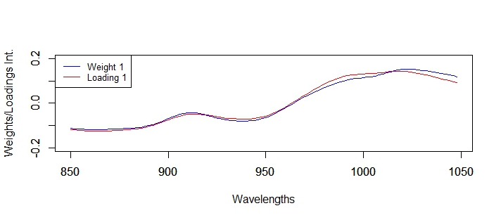
By the moment se the firsts four Loadings and Weights compared in 4 plots with the soy meal data in the conveyor:

 

 

PCR vs. PLS (part 7 - cont(b))

Apart from the Odd and Even sample Sets, I have another sample set which was fully independent from the others (samples from different origins, lab values from two different labs, and acquired in a different instrument) and I call it "Test", so we can over-plot their RMSEP  for the first 10 terms for the PLS and PCR regressions, so this way we have a, idea of the performance of the calibrations in the new instrument to which we want to transfer the calibration without using any type of standardization.

 

So we have to add some code to the previous post and change the legend:

rmsep_pls3_test_10t<-RMSEP(Xodd_pls3,ncomp=c(1:10),
                           newdata=soy_ift_test,
                           intercept=FALSE)
rmsep_pcr3_test_10t<-RMSEP(Xodd_pcr3,ncomp=c(1:10),
                           newdata=soy_ift_test
                           ,intercept=FALSE)
par(new=TRUE)
plot(rmsep_pls3_test_10t,col="orange",lwd=2,
     ylim=c(0.5,2.0),lty=4,
     axes=FALSE,type="l",
     xlab="",ylab="",main="")
par(new=TRUE)
plot(rmsep_pcr3_test_10t,col="brown",lwd=2,
     ylim=c(0.5,2.0),lty=4,
     axes=FALSE,type="l",
     xlab="",ylab="",main="")
legend("topright",legend=c("RMSECV odd PCR",
       "RMSECV odd PLS","RMSEP even PCR",
       "RMSEP even PLS","RMSEP test PCR",
       "RMSEP test PLS"),
       col=c("blue","red","blue","red",
       "orange","brown"),lty=c(1,1,4,4,4,4),lwd=2)

Finally we get this plot which is very useful to see the performance of the models:

PCR vs. PLS (part 7 - cont(a))

This post continue with the plots we have seen in PCR vs. PLS (part 7) where we saw the cross validation error for the training samples (odd samples from the soy meal), with the models developed with PCR and PLS.

 

Now we want to check how these models performs with the even samples that we have place apart in a test set.

 

Now we overlap the RMSEP statistics for the test set  (for PLS and PCR models).

#from: PCR vs. PLS (part 7)
## add extra space to right margin of plot within frame
par(mar=c(5, 4, 4, 6) + 0.1)
plot(Xodd_pcr3,"validation",estimate="CV",ylim=c(0.5,2.0),

     xlim=c(1,10),col="blue",lwd=2,
     main=" Corr & RMSEP PCR vs PLS")
par(new=TRUE)
plot(Xodd_pls3,"validation", estimate="CV",

ylim=c(0.5,2.0),xlim=c(1,10),col="red",lwd=2,
     main="")

 ## New code added

rmsep_pls3_even_10t<-RMSEP(Xodd_pls3,ncomp=c(1:10),
                           newdata=soy_ift_even,
                           intercept=FALSE)
rmsep_pcr3_even_10t<-RMSEP(Xodd_pcr3,ncomp=c(1:10),
                           newdata=soy_ift_even,
                           intercept=FALSE)
par(new=TRUE)
plot(rmsep_pls3_even_10t,col="red",
     lwd=2,ylim=c(0.5,2.0),
     lty=5,axes=FALSE,type="l",
     xlab="",ylab="",main="")
par(new=TRUE)
plot(rmsep_pcr3_even_10t,col="blue",
     lwd=2,ylim=c(0.5,2.0),
     lty=5,axes=FALSE,type="l",
     xlab="",ylab="",main="")
legend("bottomleft",legend=c("PCR-RMSECV train set",
       "PLS-RMSECV train set","PCR-RMSEP even set",
       "PLS-RMSEP even set"),
       col=c("blue","red","blue","red"),
       lty=c(1,1,5,5),lwd=1)

As we can see the Model with PLS performs better for the Even sample set and also for the cross validation.

PCR vs. PLS (Part 11) - Independent Validation

One of the interesting things of the development of a calibration for a particular application (meat meal in this case) is to install  it to work in routine and to wait for a long period of time to have a validation set which is really independent, so we can have a true statistic for the application error.

 

If you have followed the previous post, the calibration for meat meal has been developed in a DA1650, and we have used only the odd data from a sample set as training set, leaving the even samples for validation, so the calibration has almost 650 samples from the 1300 possible. The constituent we are interested to calibrate is the ash, but of course the others as protein, fat and moisture are interesting.

 

we try to develop a robust regression, so the number of terms is important and we don´t want to clean the outlier samples too much.

The range is quite wide, because we have samples from different sources (instruments, species, lab reference values,....).

 

In the previous post we saw the statistics, and they could seem quite high, but let´s see the validation.

 

The validation set is from one of the sources (one of the DA instruments, mix meat meat, and one of the labs). The samples from this source are previous to 2017, so the validation samples were acquired during 2017 and the firsts months of 2018. So this is an interesting set to check.

 

We will use the calibration (as I said) from the previous post which use 15 terms.

 

In gray we see the XY plot of the Cross Validation for the training set, and in blue how the new validation samples fit to the regression line.

gm_mult_val_plspred<-as.matrix(predict(mm_da_odd_pls,ncomp=15,newdata=gm_mult_val$NIR))
rms(gm_mult_val$Ash,gm_mult_val_plspred)
plot(mm_da_odd_pls,"prediction",ncomp=15,col="grey",
xlim=c(0,50),ylim=c(0,50))
par(new=TRUE)
plot(gm_mult_val_plspred,gm_mult_val$Ash,
xlim=c(0,50),ylim=c(0,50),col="blue",
xlab="",ylab="")
legend("topleft",legend=c("Odd 15 terms",

"VAL-2017-MIX"," VAL-2017-MIX-RMSEP 15t=1,47"),
col=c("grey","blue","blue"),pch=c(1,1,1), cex=1,
bg=)
abline(0,1)

 

It is working well in routine, and I am quite happy with the result.

 

 

PCR vs. PLS (part 10) Meat Meal

In an application for meat meal I proceed the same way as in the case of the soy meal in the Infratec. This time the instrument is a DA1650 NIR with a wavelength range from 1100 to 1650 nm. The spectra was math treated with SNV, Detrend and first derivative with data points every 2 nm. The parameter interested in for this post is the Ash.

 

Two calibration approaches had been done with the PCR and the PLS regressions. Spectra has been sorted by Ash reference value, so we can see in this plot ll the samples treated with SNV-DT and first derivative.

 

matplot(wavelength,t(NIR),type="l",
        ylab="Reflectance",
        xlab="Wavelength",
        col=AshLev)
abline(0,0)
legend("bottomleft",legend=c("0-10% Ash",
       "10-20% Ash","20-30% Ash","30-40% Ash"),
       col=c("blue","green","orange","red"),
       lty=c(1,1), cex=1)

I split the samples into odd and even , the same than in other examples and keep the even outside for external validation. The odd samples were used to develop the PCR and PLS Regressions with CV using 10 groups. Notice that the external validation with the even samples is like if we would use a CV with 2 groups.

 

Cross Validation (CV) help us to decide how many terms we would use for the development of the regression looking to the CV RMSEP graph, and in this case the graph is:

 

plot(mm_da_odd_pcr,"validation",estimate="CV",

     ylim=c(0.5,6.0),xlim=c(1,30),col="red")
par(new=TRUE)
plot(mm_da_odd_pls,"validation",estimate="CV",

     ylim=c(0.5,6.0),xlim=c(1,30),col="blue")
grid(nx = 30, ny = 6, col = "lightgray", lty = "dotted",
     lwd = par("lwd"), equilogs = TRUE)
legend("bottomleft",legend=c("PCR RMSEP","PLS RMSEP"),
       col=c("red","blue"),lty=c(1,1),cex=1)

The graph is really confuse in this case for the PCR, and we get worse results than for the PLSR. In the case of the PLSR, we see that 15 terms can be enough, but we can try with less  (10 for example) with the even validation set.

 

As we can see 15t works better than 10 for the even samples.

I have to say that in these sets there are samples from different origins, labs,...etc., and outliers have not been removed, so there is room for improvement.

PCR vs. PLS (part 7)

We have used PLS with tis data set in the posts series "Analyzing Soy Meal in transmittance", so I just want to add in these coming posts a comparison between the regresiones developed in PLS and in PCR.

 

The best way to do it is comparing some plots and in this post I show the comparison of the PCR and PLS regression with the same number of terms and with the same calibration set (odd samples), and the same validation during the development of the model (Cross Validation).

 

The plot shows how (as expected), the first terms are more correlated for the constituent of interest (protein in this case) for the PLS terms than for the PCR, so the RMS are better, but as soon as more terms are added are almost the same (a little bit better for the PLS).

## add extra space to right margin of plot within frame
par(mar=c(5, 4, 4, 6) + 0.1)
plot(Xodd_pcr3,"validation",estimate="CV",ylim=c(0.5,2.0),

     xlim=c(1,10),col="blue",lwd=2,
     main=" Corr & RMSEP PCR vs PLS")
par(new=TRUE)
plot(Xodd_pls3,"validation", estimate="CV",

ylim=c(0.5,2.0),xlim=c(1,10),col="red",lwd=2,
     main="")
## Plot the second plot and put axis scale on right
par(new=TRUE)
plot(terms,Xodd_pls3_cor,  xlab="", ylab="", ylim=c(0,1),
     axes=FALSE, type="l",lty=4,lwd=2, col="red")
par(new=TRUE)
plot(terms,Xodd_pcr3_cor,  xlab="", ylab="", ylim=c(0,1),
     axes=FALSE,type="l",lty=4,lwd=2, col="blue")
## a little farther out (line=4) to make room for labels
mtext("Correlation",side=4,col="black",line=3)
axis(4, ylim=c(0,1), col="black",col.axis="black",las=1)
legend("bottomright",legend=c("RMSEP PLS", "RMSEP PCR",

       "Corr PLS","Corr PCR"),
       col=c("red","blue","red","blue"),

       lty=c(1,1,4,4),lwd=2)

 A reason for the improvement in the PLS can be seen in the regression coefficients (with 5 terms), where the PLS (in red), are more sharp, and can give better estimations ( we try to analyze this in coming posts)

 

PCR vs. PLS (Part 6)

After checking the RMSEP and correlation with different terms in the PCR I get this plot:

using this code:
par(mar=c(5, 4, 4, 6) + 0.1)
plot(Xodd_pcr3,"validation",estimate="CV",
     col="blue",ylim=c(0.5,2.5),
     xlim=c(1,10),lwd=2,xlab="",ylab="",main="")
par(new=TRUE)
plot(terms,Test_rms,type="l",col="red",ylim=c(0.5,2.5),
     xlim=c(1,10),lwd=2,xlab="Nº Terms",
     ylab="RMSEP",
     main=("CV vs Ext Validation & Corr"))
## Plot the second plot and put axis scale on right
par(new=TRUE)
plot(terms, Test_corr, pch=15,  xlab="", ylab="",
     ylim=c(0,1),axes=FALSE, type="b", col="green")
## a little farther out (line=4) to make room for labels
mtext("Correlation",side=4,col="green",line=3)
      axis(4, ylim=c(0,1), col="green",
      col.axis="green",las=1)
legend("topright",legend=c("CV", "Ext Val","Corr"),
       col=c(1:3),lwd=2)
## In the plot 5 seems to be the best option
   for the number of terms

 

Now we can compare the results in the XY plot, as we saw in the post "PCR vs. PLS (part 5)" to get the conclusions.

The statistics for this external validation set with 5 terms are (Monitor function):

> monitor10c24xyplot(pred_vs_ref_test_5t)
Validation Samples  = 25 
Reference Mean  = 45.6236 
Predicted Mean  = 46.38495 
RMSEP    : 1.046828 
Bias     : -0.761354 
SEP      : 0.7332779 
Corr     : 0.9131366 
RSQ      : 0.8338185 
Slope    : 0.7805282 
Intercept: 9.418837 
RER      : 8.115895   Poor 
RPD      : 2.428305   Fair 
Residual Std Dev is : 0.633808 
    ***Slope/Intercept adjustment is recommended***
BCL(+/-): 0.3020428 
***Bias adjustment in not necessary***
Without any adjustment and using  SEP as std dev 

the residual distibution is: Residuals into 68% prob (+/- 1SEP) = 15 % = 60 Residuals into 95% prob (+/- 2SEP) = 21 % = 84 Residuals into 99.5% prob (+/- 3SEP) = 23 % = 92 Residuals outside 99.5% prob (+/- 3SEP) = 2 % = 8 With S/I correction and using Sres as standard deviation,

the Residual Distribution would be: Residuals into 68% prob (+/- 1Sres) = 20 % = 80 Residuals into 95% prob (+/- 2Sres) = 24 % = 96 Residuals into 99.5% prob (+/- 3Sres) = 25 % = 100 Residuals outside 99.5% prob (> 3Sres) = 0 % = 0

Selecting samples for lab analysis (part 4)

After the last post, we have a training set with 30 samples to develop a calibration (due to the few samples, this exercise is just a study in order to create a model with more samples in the future), and a test set with another 30 samples. This test set is useful to tune the model as best as we can (math treatments, number of terms,...).

We just try with the parameter protein, developing a PLSR with the Training Set, and after that predicting the Test set. The prediction values for the Test Set are compared with the Test Set Lab values in order to get the performance statistics.

Validation statistics are compared with the Regression statistics.

Finally a model with the Training + Test Set is developed (60 samples).

All the statistics are studied with a monitor function.

See the script and follow the tutorial in Github.

Details of the plots in the monitor function: