Quadratic trendlines

In the last post, I talk about the use of the function "detrend" in the package "prospectr" to remove the quadratic trend lines in the soil NIR spectra. We can see these trendlines overplotted to the spectra (I do it just for five of the soil spectra from the Spanish soil LUCAS database).

In red is the spectra treated with SNV and in blue the quadratic trend lines to apply to the SNV treated spectra, to remove them and convert them in a SNV + Detrend spectra.

Working with Soilspec data (part 8)

We continue in this post with the "chemometrics" package used in the previous one. Indeed the ellipses here we see the cutoff and the samples which are bellow and over it. 

Apart from the graphics we can have a list with the sample number and the robust or classical Mahalanobis distances values.

Is it interesting to see the distribution of the Mahalanobis distances, and for that we can use the histograms:

hist(res$md)    (classical Mahalanobis distance)
hist(res$rd)    (robust distance)

Normally we see the classical histogram in the software we commonly use, due that they use the classical Mahalanobis distance.

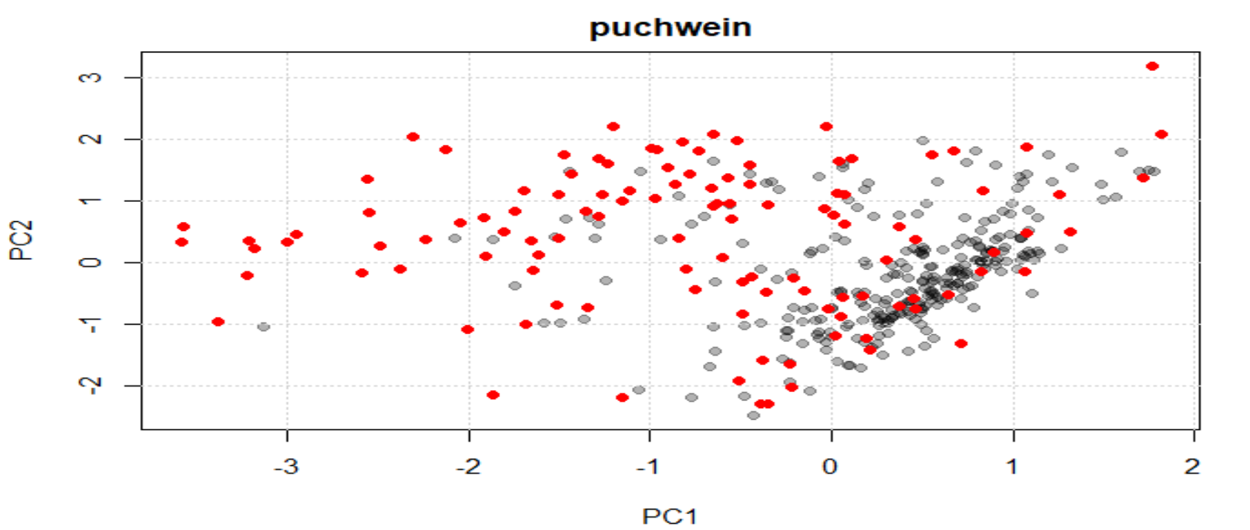
Now it is time to reduce the database to take the structure of it, this way can serve to us to send the selected samples to the lab and to save money in the development of the calibration and at the same time keep the variability of the samples. There are several algorithms to do it with the “prospectr” package, being one of then the ShenkWest (nice to have this algorithm in R, and all that workm with Win ISI know it quite well), but I am going to use the “puchwein”, because it seems to me that it capture the structure quite well.

pu <- puchwein(X = PC_scores, k = 0.1, pc =5) 

plot(pu$pc[,c(1,2)], col = rgb(0, 0, 0, 0.3), 

     pch = 19, main = "puchwein")
grid()
points(pu$pc[pu$model,],col = "red", pch = 19) 

Now we can see the selected samples in the scores map PC1 vs PC2 in red color. These samples keep the structure quite well and can be used to send them to the lab.

Quimiometria con R: Trim Spectra

Quimiometría con R: PUCHWAIN Algorithm

Mahalanobis in PC space (removing redundat)

In a previous post, we used "prospectr", with the duplex function to select a training set (30 samples), in order to spend less money in lab analysis. This way, we remove redundants spectra, and the selected spectra are well dispersing all around the PC space. Redundant were discarded according to its Neighborhood Mahalanobis distance.

In this plot, we can see the selected samples (red ones), and a Mahalanobis ellipse, considering all the samples with the "drawMahal" function from the package "chemometrics".

If we consider just the red samples (the 30 samples for the training set), the center of the population will be different that with all the samples (156), so we have to calculate the PCs again (their orientation will change), and we can draw a new Mahalanobis  ellipse (97.5 quantile).

As we can see in the plots,  removing the redundantswill give more weigth to the extreme samples, to be retained, and not be consider as outliers.

Selecting samples for lab analysis (part 3)

I have been using 159 spectra of soya meal in order to select 60 of them to send to the laboratory (imagine that I can only afford to analyze this number due to the high cost of the reference methods). It is obvious that I would like to select a set which represent as better as possible the whole population of these 159 samples. I used the “duplex algorithm" from "prospectr package", which select a “model set” and a “test set”, so I will have 30 on each.

Some days later the result from the “Lab” are here, so I am anxious to check the “summary” and the “histograms”. Normally you have an idea of the range of protein in the soya meal that you received, and this can help you to check if the sample sets are representative. But in this case I have the advantage to have all the lab values for the 159 samples, so let´s see: (green: Histogram of the 159 samples for protein, blue:histogram of the 30 samples for training, violet: histogram of the 30 samples for validation).

             

Some script using "prospectr"

library(prospectr)
hsoja.X<-as.matrix(read.table("clipboard",header=FALSE))
wavelength1<-seq(from=1100.0,to=2499.5, by=0.5)
X.ID<-seq(from=1,to=159, by=1)
colnames(hsoja.X)<-wavelength1
rownames(hsoja.X)<-X.ID
plot(as.numeric(colnames(hsoja.X)),hsoja.X[1,],
   +type="l",xlab="wavelength",ylab="Absorbance")
matplot(wavelength1,t(hsoja.X),type="l")
hsoja.X.bin<-binning(hsoja.X,bin.size=4)
wavelength2<-seq(from=1100,to=2498, by=2)
colnames(hsoja.X.bin)<-wavelength2
matplot(wavelength2,t(hsoja.X.bin),type="l",
ylab="",xlab="Wavelength")
points(as.numeric(colnames(hsoja.X.bin)),
   +hsoja.X.bin[1,],pch=2)
matplot(wavelength1,t(hsoja.X),type="l",ylab="",
   +xlab="Wavelength",col="black")
par(new=T)
hsoja.Xsnv<-standardNormalVariate(X=hsoja.X)
matplot(wavelength1,t(hsoja.Xsnv),type="l",xaxt="n",
   +yaxt="n",ylab="",xlab="",col="blue")
hsoja.Xsnvdt<-detrend(X=hsoja.X,wav=as.numeric(colnames(hsoja.X)))
par(new=T)
matplot(wavelength1,t(hsoja.Xsnvdt),type="l",
xaxt="n",yaxt="n",xlab="",ylab="",col="red")
h.soja.snvdt1d<-t(diff(t(hsoja.Xsnvdt),differences=1,lag=16))
wavelength3<-seq(from=1108,to=2499.5, by=0.5)
par(new=T)
matplot(wavelength3,t(h.soja.snvdt1d),type="l",
   +xaxt="n",yaxt="n",xlab="",ylab="",col="green")
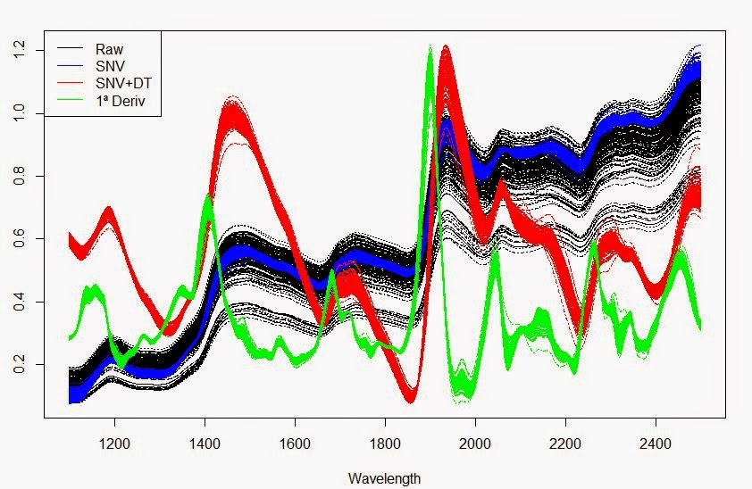
# All the sequence for the plot
matplot(wavelength1,t(hsoja.X),type="l",
   +ylab="",xlab="Wavelength",col="black")
par(new=T)
matplot(wavelength1,t(hsoja.Xsnv),type="l",
   +xaxt="n",yaxt="n",ylab="",xlab="",col=4)
par(new=T)
matplot(wavelength1,t(hsoja.Xsnvdt),type="l",
   +xaxt="n",yaxt="n",xlab="",ylab="",col=2)
par(new=T)
matplot(wavelength3,t(h.soja.snvdt1d),
   +type="l",xaxt="n",yaxt="n",xlab="",ylab="",col="green")
legend("topleft",legend=c("Raw","SNV","SNV+DT","1ª Deriv"),
   +lty=c(1,1),col=c("black","blue","red","green"))

Reducing the X matrix (Binning)

There are situations where we have spectra with a huge amount of data points and we want to reduce the number of them. There are instruments which measure spectra every 0.5 nm. This is an important advance in order to make instruments more similar one to the other in the wavelength scale, so the transferability is better, but this feature does not represent and advance when we are developing a model or calibration. In this case the normal procedure is to reduce the number of data points.

Continue using the “prospectr” package we have a function which can help us to do this task.

The steps I follow for this task, were:

1.   I exported a CAL file from Win ISI (just the NIR segment) to Excel.

2.   I copied the Matrix from Excel into the Clipboard.

3.   I use this code to imported the X matrix into R:

hsoja.X<- as.matrix(read.table("clipboard",header=FALSE))

The dimension of this X matrix is: (159,2800), the number of samples is 159 and the number of wavelengths 2800. In the case that we have used a NIR instrument which acquires data points every 2 nm, the matrix would be (159,700), so the idea is to reduce the Matrix to this size.

plot(as.numeric(colnames(hsoja.X)),hsoja.X[1,],type="l",

+ xlab="wavelength",ylab="Absorbance")

4.   Now we use the “binning” function to reduce the matrix, keeping one data points every a certain number (bin.size).In this case we will use a bin size of 4, in order to have 2800:4 = 700 data points.

hsoja.X.bin<- binning(hsoja.X,bin.size=4)

5.   Now we can work with a more reduce X matrix.