Mostrando entradas con la etiqueta LUCAS database. Mostrar todas las entradas

12 jul 2022

NIR RMS between subsamples

One of the advantages of R, is that you can develop a function to apply to your calculations to get your purpose. In this case I wanted to apply the RMS calculation to every row of the difference matrix we have seen in the previous post.

We can see with an histogram the distribution of the RMS values


11 jul 2022

Diference between subsamples

Once we have sorted and grouped all the samples and subsamples, we can create two matrices one that contains the odd samples (first subsample) and other with the even subsamples (second subsample), this way we can calculate the spectra difference between subsamples and check the spectra.

This difference spectra matrix is important to calculate the RMS between subsamples, that gave us an idea how similar are the subsamples between them. Just sum the squared values for every spectrum difference, divide by the number of wavelengths and calculate the square root.


6 jul 2022

Soil clay regressions: Looking for the better accuracy (part 3)

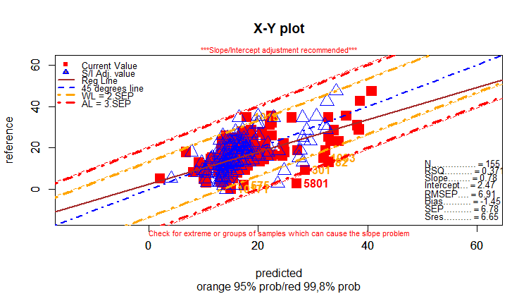
 Now we have four calibrations for clay in soil developed with a selection of samples from the LUCAS database (Spanish crop soils). Now we want to see if those calibrations predict with certain accuracy a new set of soil samples (155) from a Spanish region, acquired in a different instrument and at a different laboratory.

In these cases, it is normal to expect a bias or a slope in the predictions, so we can use the model with those adjustments applied, until the database is updated and a new expanded method with new variability (instrument, laboratory, region,) developed.

Well, these are the results of the XY plots  "Lab vs Predictions" for this independent data set:

PLS predictions:


Random Forest Predictions

Cubist Predictions


MBL Predictions


As we see in all the cases some adjustment or calibration update is needed. We can try to reprocess everything trying to find a better configuration which improves these values, but in that case this new set will never be independent again like it is now. 


5 jul 2022

Soil clay regressions: Looking for the better accuracy (part 2)

Let´s select a seed (to fix the training and test set) and develop the regression with four algorithms (PLS, Random Forest, Cubist and Memory Based Learning.

These are the Test Validation XY plots and statistics:

PLS Regression:


Random Forest Regression:


Cubist Regression:


Memory Based Learning Regression


We can see PLS give the better RMSEP, but some samples are outside the Action Limits Warning, while that in the MBL the residual distribution is more stable and there are no samples outside the action limits threshold.

4 jul 2022

Soil clay regressions: Looking for the better accuracy (part 1)

To have a good traceability in our data bases is important to develop accurate calibrations. We have seen with the Soil LUCAS database that we can filter the data by sample origin (Spain for my case) and after that filter it by land type (I choose for this example “Croplands). The samples are split into training and test set randomly.

 After that we must decide if we choose all the wavelength range (VIS + NIR) or the just the NIR. In this case the calibration is for Clay and different test tell me that the complete range is the best option.

 After this is time to check for the best math treatment trying in this case with 2º SG derivative, 1º SG derivative and SNV+Detrend scatter correction. The last two options gave me better validation statistics than the 2º SG derivative when using a PLS regression

 This is the XY plot for the validation set:


Can we improve the results with another type of regression for these cropland samples? This is what we will see in the next coming posts.

Another question can be: May I use this database to predict samples from another database? These can be samples from a different area in the same country, taken with a different instrument and analysed in a different laboratory. Check all this is important to see the robustness of the calibrations.


21 feb 2022

To consider for the Mahalanobis distance calculation

 As we saw in the post "Try to find high content gypsum samples (part 3)" , when we develop the principal component analysis as much variance as possible (we determine the explained variance limit) is explained, and unless we saw all the sores maps, we may have not a good idea about what is happening to our data.

The average spectrum represents all the groups, so we cannot expect that with the Mahalanobis distance all the samples with gypsum will be marked as outliers, because the average spectrum represents as well those samples. Only the ones with high and very high gypsum content can probably be marked as outliers by Mahalanobis distance. Now that we have make two samples sets ("gypsum content" and "non or low gypsum content"), we can check the sample sets separately to understand better our data.

Let´s check again the Mahalanobis distance plot once we have, by spectra visualization and discrimination by correlation, the two sample sets ("No" and "Yes" gypsum content):


See how some of the gypsum content samples are over 3 Mahalanobis cut-off (but not all).
Now that the "No" samples are in a new sample set, we can see their spectra:

There are some samples that seem outliers, but all the rest seem to group quite well together, anyway we wait to see the PC score maps:
Now we see different patterns.

Let´s see finally the new Mahalanobis distances:


7 feb 2022

Trying to find high content gypsum samples (part 3)

 If we go back to the post: "PCA with the first derivative" we saw how there was some groupings (in the PC2 vs. the rest PC maps) in the scores, after, when looking to second loading we though that could be the samples with gypsum content. 

In the last two posts : "Trying to find high content gypsum samples (part 1)" and "Trying to find high content gypsum samples (part 2)",  we found those samples by correlation with a Gypsum reference spectra, and now we can create a new variable called "gypsum" which takes the factor value "Yes" or  "No", so now we can see easier in the score maps if that grouping was due to the content of gypsum:

pairs(scores_1df[ ,1:6], col = scores_1df$gypsum)


6 feb 2022

Trying to find high content gypsum samples

How can I find the high content gypsum samples in the LUCAS spanish database?. We have the spectrum of pure gypsum, so we can try to correlate (or meassure a distance) every spectrum of the database with the pure gypsum spectra and see if we find some threshold or gap that splits these high content gypsum samples. 

I try in this case the correlation, because it is the easiest algorithm, and  I don´t have a population of gypsum soil spectra (just one reference pure spectrum).

Let´s run the correlation:

corSG1 <- as.numeric(cor(t(lucas_spain$spcnir_SG[,21:546]),
                     mineralRef_nir_2nm_SG1[3, 21:546]))

Now we have a correlation value for every spectrum, so we can plot the histogram:

hist(corSG1, breaks = 1000)

We can see the distribution and the tail on the right with some grouping over 0.85, so this can be a way to look at the samples over 0.8 correlation and make a fine tune selection.

24 ene 2022

PCA with the first derivative

In a previous post we had calculated the PCA with the math treatment SNV+Detrend and we calculated a first sample set of outliers with the Mahalanobis distance. 

When calculating PCA we have to treat as best the spectra as possible in order to detect populations or boundaries and if we treat the spectra with math treatments which help to do this task is great. So indeed, to apply the SNV + Detrend, I apply this time the first derivative to the spectra (soil from Spanish soil from LUCAS database) and calculate the PCA.

We can have a look to the score’s maps (six PC recommended) to find if there are boundaries on them:

Look at the maps which include PC2 as one of the axes. There are a certain number of samples which takes a different direction than the rest. This second PC term can be useful to find something interesting on the spectra.

 To see what is happening we can see the loading spectra for this second PC term:

This loading spectra has the first derivative math treatment applied, so we can compare it with a library of reference known spectra (minerals in this case) to see which is the best match, and in this case the best match is with the gypsum mineral, so this second term is explaining part of the variance included in our spectra database due to the addition of gypsum to the soil.


23 ene 2022

LUCAS SP Database vs. pure mineral Gypsum

In order to find if the soil has traces of a certain mineral, it is useful to overplot our soil samples (in this case the soil Spanish samples included in the LUCAS database, with the pure mineral spectrum  (in this case Gypsum). We must  overplot them with the same math treatment and in the same scale. I do it, in this case, with the spectra treated with the SG second derivative.


 In red is the pure gypsum mineral and in grey samples in the soil database.  As we can see some of the bands match, so we can be quite sure that there are some samples in the database with gypsum content to certain levels.

Second derivative is quite helpfull to find these matches. If we do it, for example with SNV+Detrend, some of the bands are hiden by other samples and the assumption that there are samples with gypsum is less clear.


13 ene 2022

Detecting outliers with Mahalanobis distance

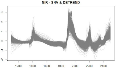
In this first plot we see the spectra of the LUCAS spanish database treated with the SNV and Detrend math treatment of the "Prospectr" package, where we remove the quadratic trend (as we saw in the last post):


The next step is to calculate the Principal Components Analysis, where we calculate the scores of every sample for the selected components. These scores are stored in a score matrix, which have a centre.

The next step is to measure the distance from every sample projected in the PC space to this centre. This distance (calculated with the function "fdiss" from the "resamble" package) can be represented in a plot aconsidering the spectra with distances higher than 3.00 as outliers.


Which are this samples? just mark them on the first plot and take out some conclusions:


As we can see they seem to be quite different of the average spectrum (considered the center), but we can consider that there are other samples which are not selected as outliers and they seem to be. 

The normal procedure is to remove in a first step these samples, and calculate again the new centre with the rest and proceed with a new mahalanobis distance calculation


11 ene 2022

Quadratic trendlines

In the last post, I talk about the use of the function "detrend" in the package "prospectr" to remove the quadratic trend lines in the soil NIR spectra. We can see these trendlines overplotted to the spectra (I do it just for five of the soil spectra from the Spanish soil LUCAS database).

In red is the spectra treated with SNV and in blue the quadratic trend lines to apply to the SNV treated spectra, to remove them and convert them in a SNV + Detrend spectra.


5 ene 2022

Trim spectra from LUCAS database

The spectra from LUCAS database (ESDAC*) seem to come from a XDS  (VIS + NIR) instrument, and this instrument give two options when exporting the spectra (every 0.5 nm, and every 2 nm), the data comes in 0.5 nm, and that means that we have 4200  data poits per spectrum, and that means a huge spectra matrix.

We can trim the spectra keeping just the spectral data every two nanometers, so we will have the reflectance values from 400 to 2498 nm every 2nm, so we have a less heavy matrix of 1050 data points per spectrum. This fuction will give us the spectra like a NIR6500.

Just create a sequence to select one column of every four, and call that function (like in my case) "trim05to2":

dim(lucas_spain$spc)
 2604 4200

spec2nm <- trim05to2(lucas_spain$spc)

dim(spec2nm)
 2604 1050


*European Soil Data Centre (ESDAC), esdac.jrc.ec.europa.eu, European Commission, Joint Research Centre

Importing LUCAS database from R into WinISI


Once we have the spectra we want from the LUCAS database (ESDAC*) in R, we can export it to a "txt" file with:


write.table(spec2nm, file="lucas_spain.txt",
            row.names=TRUE,
            col.names=FALSE)


This way we have the samples IDs, but we don´t need the column name (wavelengths), because Win ISI will create them when importing the spectra.


Once we have the txt file, we convert it to a ".nir" file which is the spectra format for Win ISI with the Win ISI tool "Convert", selecting the configuration from TXT to Win ISI.

After filling  the options Win ISI ask, we wait for the conversion succeeded message and we have the ".nir" file ready to view:


Now we do the same with the parameters (constituents) we are interested in:

write.table(lucas_spain[ ,c(1, 5:16)],                                           file="lucas_spain_constituents.txt", 
            row.names=TRUE, col.names=TRUE)

We export the samples IDs as well, to link them with the spectra. Finally we import the parameters to the spectra to get the ".cal" file and ready to work with the spanish LUCAS database in Win ISI.

*European Soil Data Centre (ESDAC), esdac.jrc.ec.europa.eu, European Commission, Joint Research Centre