Descarga y trabaja con datos de suelos en NIR

 Una de las páginas donde te puedes descargar datos de espectros de suelos con sus métodos de referencia es en 

ZENODO: Agroscope_SoilSpectralLibrary_2024.

You can download soil spectra analysis to work with from:

ZENODO: Agroscope_SoilSpectralLibrary_2024

Digital Soil Spectroscopy

Standard Normal Variate (SNV)

 As in previous posts, we are going to follow the Soil spectroscopy training material and we are going to use the reference material provided.

Let´s start loading the libraries and the data:

library(tidyverse)
library(prospectr)
load("C:/BLOG/Workspaces/NIR Soil Tutorial/post5.RData")

In the training material we can read a clear explanation of what SNV does:

“Standard normal variate is a simple and widely used method that works by centering each individual spectrum to zero and then dividing each spectral band value by the standard deviation of the entire spectrum. The SNV method processes each observation independently. The disadvantage of SNV is that it can be sensitive to noise”.

So for each spectrum we calculate the mean of all data points reflectance values and also their standard deviation. Then we subtract for every data point the mean and divide the result by the standard deviation.

Using the prospectr package, we can use the standardNormalVariate function to apply the SNV transformation to the spectra matrix.

snv_spectra <- standardNormalVariate(dat$spc)

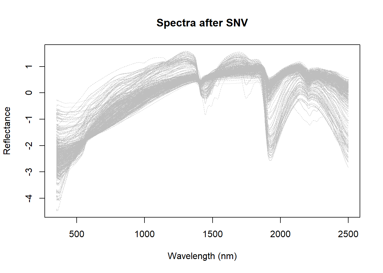
Let´s use first classical R function matplot to plot the spectra before and after the SNV transformation:

matplot(colnames(dat$spc),
  t(snv_spectra),
  type = "l",
  col = "grey",
  lwd = 0.5,
  xlab = "Wavelength (nm)",
  ylab = "Reflectance",
  main = "Spectra after SNV"
)

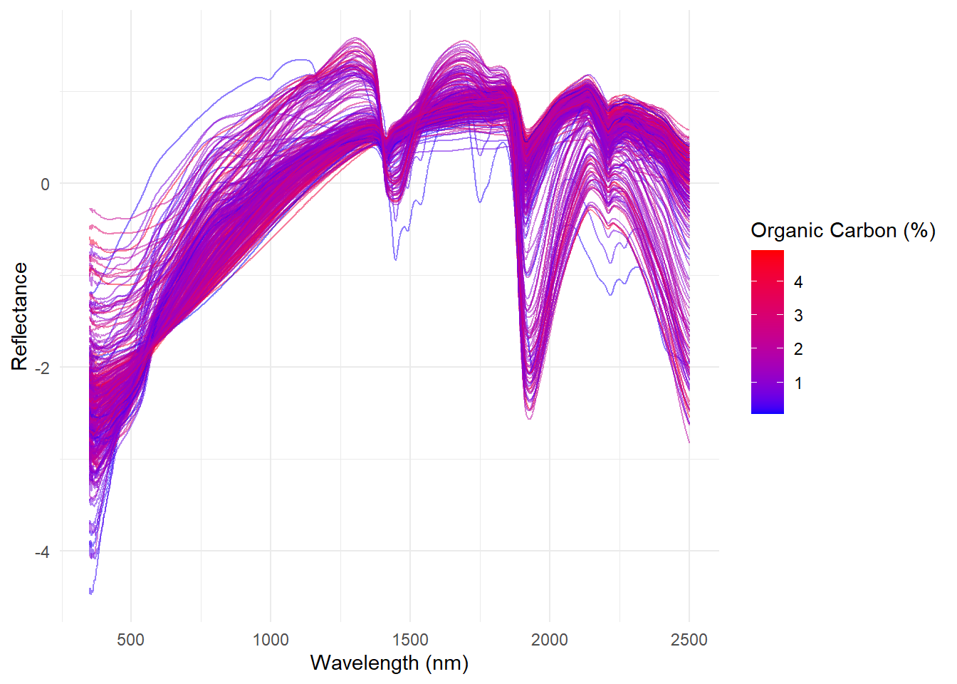
Now with ggplot2:

# Create the long-format data frame for the different derivatives
snv_spectra_long <- data.frame(
sample = rep(1:nrow(dat), each = ncol(snv_spectra)),
oc = rep(dat$Organic_Carbon, each = ncol(snv_spectra)),
clay = rep(dat$Clay, each = ncol(snv_spectra)),
silt = rep(dat$Silt, each = ncol(snv_spectra)),
sand = rep(dat$Sand, each = ncol(snv_spectra)),
wavelength = rep(my_wavelengths, nrow(snv_spectra)),
absorbance = as.vector(t(snv_spectra))
)


ggplot(snv_spectra_long, aes(x = wavelength, y = absorbance, 
                             group = sample, color = oc)) +
  geom_line(alpha = 0.5) + # Set alpha to 0.5 for transparency
  scale_color_gradient(low = 'blue', high = 'red') +
  theme_minimal() +
  labs(x = 'Wavelength (nm)', y = 'Reflectance', color = 'Organic Carbon (%)')

Bibliography:

Soil spectroscopy training material Wadoux, A., Ramirez-Lopez, L., Ge, Y., Barra, I. & Peng, Y. 2025. A course on applied data analytics for soil analysis with infrared spectroscopy – Soil spectroscopy training manual 2. Rome, FAO.

NIR Chemometrics for soil analysis

Adding noise to the spectra

 We have seen in the previous post how to remove artifacts in the spectra using the spliceCorrection function from the prospectr package. But there are other sources of noise in the spectra which depends of several factors, as the quality of the spectrophotometer (can use a signal to noise ratio meassurement to test it), the scanning time, resolution, sample presentation, …. In this post we continue with the “course on applied data analytics for soil analysis with infrared spectroscopy” using the reference material provided. And this time we are going to see the part of the course where we add noise to the spectra and then we apply two methods to remove it. The methods are the Moving Window Average and the Savitzky-Golay Filter.

First we load the libraries we are going to use:

library(tidyverse)
load("C:/BLOG/Workspaces/NIR Soil Tutorial/post4.RData")

Adding noise to the first spectrum

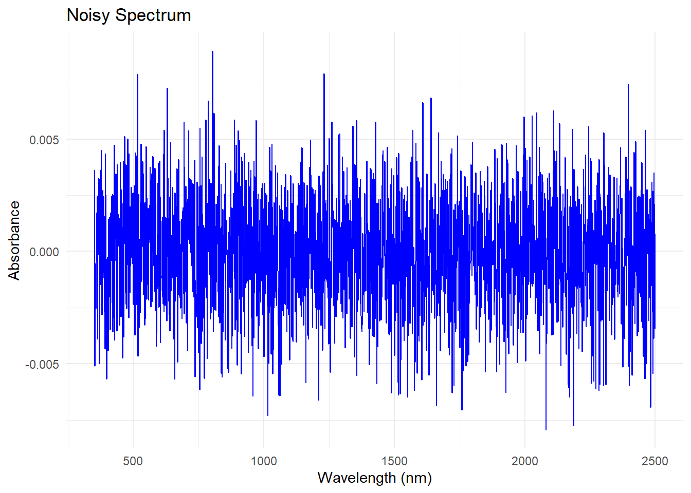
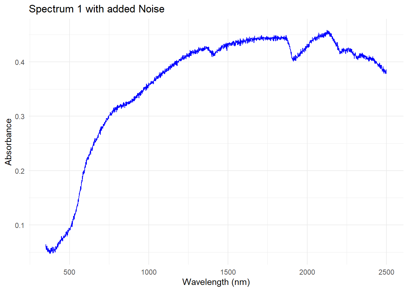
We create some Gaussian noise to the first spectrum in the dataset (mean = 0, standard deviation = 0.0025), and we are gong to add it to the first spectrum in the dataset. Take in account that we are going to select the dataset dat$spc, which is the one we created in the previous post, so we are going to use the spectra without the artifacts.

#Set a seed for reproducibility of random noise
set.seed(801124)
# Add random noise to the first sample’s spectrum
my_noisy_spc <- dat$spc[1, ] + rnorm(ncol(dat$spc), sd = 0.0025)

If we just want to se the noise that we are adding:

ggplot(data = data.frame(wavelength = my_wavelengths, absorbance = rnorm(ncol(dat$spc), sd = 0.0025)),
       aes(x = wavelength, y = absorbance)) +
  geom_line(color = "blue") +
  labs(title = "Noisy Spectrum",
       x = "Wavelength (nm)",
       y = "Absorbance") +
  theme_minimal()

Plotting the noisy spectrum

ggplot(data = data.frame(wavelength = my_wavelengths, absorbance = my_noisy_spc),
       aes(x = wavelength, y = absorbance)) +
  geom_line(color = "blue") +
  labs(title = "Spectrum 1 with added Noise",
       x = "Wavelength (nm)",
       y = "Absorbance") +
  theme_minimal()

Removing the noise

No let´s apply to this spectrum two methods used to remove noise:

Moving Window Average

library(prospectr)
# Replace ‘my_noisy_spc’ with your actual data frame or matrix and ‘w’ with the desired
# window size
mwa_result <- movav(my_noisy_spc, w = 11)

Savitzky-Golay Filter

# Replace ‘my_noisy_spc’ with your actual data frame or matrix, ‘m’ with the window size,
# and ‘p’ with the polynomial order
sg_result <- savitzkyGolay(
my_noisy_spc, # the noisy spectrum
m = 0, # this m is for the derivative order, 0 is for no derivative
p = 3, # the polynomial order
w = 11 # the window size
)

# Create a long-format data frame for the MVA spectrum
long_mwa_spc <- data.frame(
wavelength = as.numeric(names(mwa_result)), # Extract the wavelengths
spectral_value = mwa_result, # Store the spectral values from the MVA
method = 'mva' # Label the data
)
# Create a long-format data frame for the Savitzky-Golay (SG) spectrum
long_sg_spc <- data.frame(
wavelength = as.numeric(names(sg_result)), # Extract the wavelengths
spectral_value = sg_result, # Store the spectral values from the SG
method = 'sg' # Label the data
)
# Combine the long-format MVA and SG data frames into one
denoised_long <- rbind(long_mwa_spc, long_sg_spc)

Now we create a data frame for the original noisy spectrum and some labels.

# Create a data frame for the original noisy spectrum
original_noisy <- data.frame(
wavelength = my_wavelengths, # Use the original wavelengths
spectral_value = my_noisy_spc # Use the original noisy spectrum values
)

my_labels <- c(
'mva' = 'Moving average smoothing',
'sg' = 'Savitzky-Golay filtering'
)

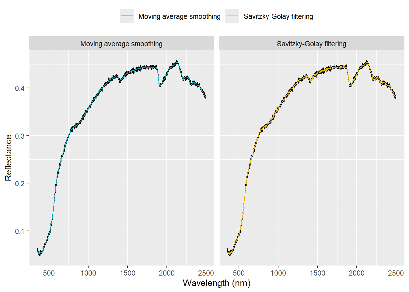
Now we want to overplot the corrected spectra over the noisy one:

# Plot the spectra using ggplot2
ggplot() +
# Plot the original noisy spectrum as a red line in the background
geom_line(
data = original_noisy,
aes(x = wavelength, y = spectral_value),
color = 'black'
) +
# Plot the MVA and SG processed spectra on top of the original noisy spectrum
geom_line(
data = denoised_long,
aes(x = wavelength, y = spectral_value, color = method, group = method)
) +
# Add titles and labels for the axes
labs(
x = 'Wavelength (nm)',
y = 'Reflectance'
) +
#coord_cartesian(xlim = c(1500, 1800), ylim = c(0.425, 0.450)) +
# Manually set the colors for the MVA and SG lines
scale_color_manual(
values = c('mva' = '#00AFBB', 'sg' = '#E7B800'),
labels = my_labels
) +
# Facet the plot by the method, creating separate plots for MVA and SG
facet_grid(. ~ method, labeller = labeller(method = my_labels)) +
theme(legend.position = 'top') + guides(color = guide_legend(title = NULL))

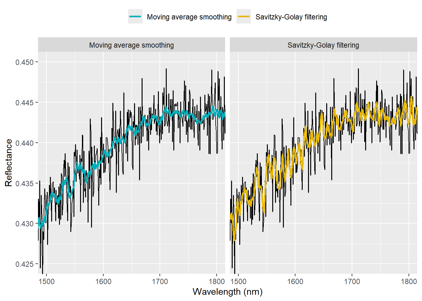
We can zoom the spectra to see the differences more clearly:

ggplot() +
# Plot the original noisy spectrum as a red line in the background
geom_line(
data = original_noisy,
aes(x = wavelength, y = spectral_value),
color = 'black'
) +
# Plot the MVA and SG processed spectra on top of the original noisy spectrum
geom_line(
data = denoised_long,
aes(x = wavelength, y = spectral_value, color = method, group = method), size = 1
) +
# Add titles and labels for the axes
labs(
x = 'Wavelength (nm)',
y = 'Reflectance'
) +
coord_cartesian(xlim = c(1500, 1800), ylim = c(0.425, 0.450)) +
# Manually set the colors for the MVA and SG lines
scale_color_manual(
values = c('mva' = '#00AFBB', 'sg' = '#E7B800'),
labels = my_labels
) +
# Facet the plot by the method, creating separate plots for MVA and SG
facet_grid(. ~ method, labeller = labeller(method = my_labels)) +
theme(legend.position = 'top') + guides(color = guide_legend(title = NULL))

Bibliography:

Soil spectroscopy training material Wadoux, A., Ramirez-Lopez, L., Ge, Y., Barra, I. & Peng, Y. 2025. A course on applied data analytics for soil analysis with infrared spectroscopy – Soil spectroscopy training manual 2. Rome, FAO.