Searching / Archiving samples in ISI Scan

All the samples in ISI Scan are stored in the "data" folder in the ISI Scan directory. Keeping the Access data base, and  files included into that data folder is important to run the ISI Scan fast and secure.

So it is important to make backups regularly and clean the database at the same time. All this is configures at the System Profile window.

 

In this window, we configure the samples the samples which stay in the database and the samples which are exported or deleted definitively.

Spectra of samples with Lab Value attached are always kept in ISI Scan , so they can be exported as CAL files or used for Monitor purposes.

Read the ISI Scan Help section of System profile for a better understanding of the procedure.
After the Backup, a window appears searching for samples to archive:

Samples are archived in a new folder called Archive inside the Backup folder. Into this Archive folder there are new folders with the name of the products and inside this folders are the NIR files with the spectra, and the ANL or CSV files with the results. So you can export this files to Win ISI to work with them.

 

If the samples stay in the Data folder of ISI Scan and are not yet archived, we can search them clicking with the mouse on Products and selecting "Search". A new window appears where we have filter options, once searched the samples will go to the "Selected Samples" folder.

 

 

Merry Christmas from NIR-Quimiometria

Hello dear readers.

Thanks to all of you for your support , and I wish you a very nice Chistmas time.

2 ways to draw a spectra set with plot 3D

Reading the article "Fifty ways to draw a volcano using package plot3D",

I wanted to test it with spectra (in this case treated with SNV). The result looks nice, but I have to practice more with it.

It seems that there are nice applications to use these plots in Chemometrics for tutorials, so more ideas are coming how to use them.

persp3D(z = X2.val_snv, facets = FALSE, col = "darkblue")

> persp3D(z = X2.val_snv) 

Plots to check the STD

 

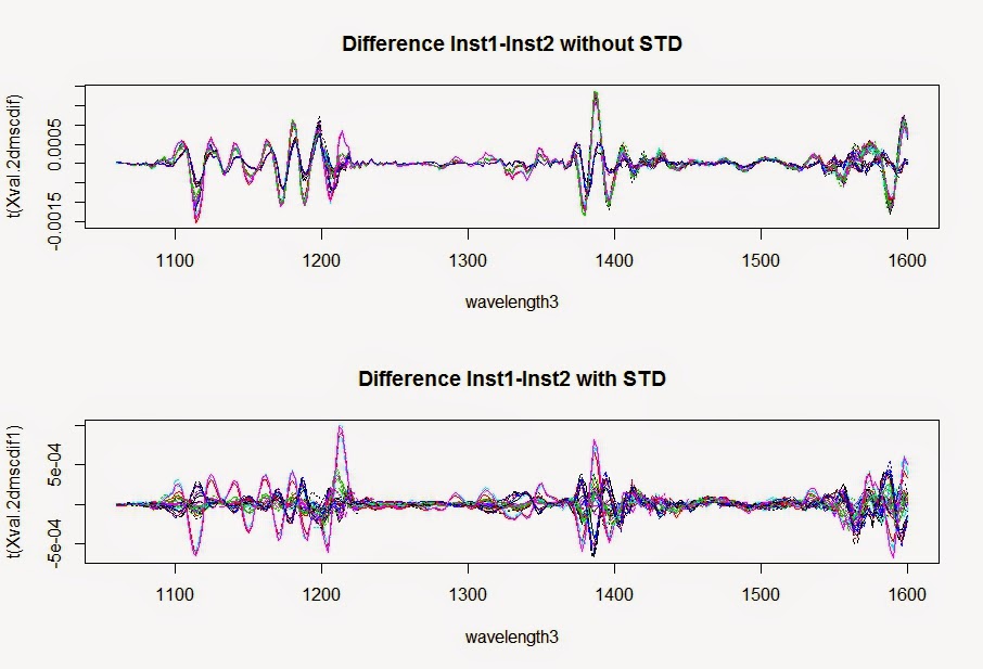
Spectra plots also will help us to understand how the STD correct the spectra, looking to the spectra and study the patterns we can see for wich samples works better or worse. We expect to see as much random noise as possible.

These plots are the validation samples of the Shootout 2002, with a standardization developed with a factor matrix multiplied to the unstandardized validation spectra. As said in previous posts, 8 samples were selected, but other samples could give (or not) similar plots.

Selection of samples is an important task. What is clear is that with the STD applied we get much better statistics as we saw in the post: "Standardizing the spectra (Shootout 2002)".

 

 

 

 

Plots to prepare the STD

In the previous post 8 samples were selected for the STD.

First figure shows the selected samples for the STD scanned (raw spectra) in Instrument 1 and 2, and the differences between them.

 

We can see the same procedure, but in this case the comparative is done with math-treatments (2º Derivative + MSC). As expected much more peaks in the spectra of the difference:

 

In a recent article from Mark Westerhaus to NIR News, he advice about the importance to check and review these plots and its shape, in order to apply the best standardization (single or multiple).

Comparing with more details the spectra, there are differences in the instruments not only in the photometric scale, also in the wavelength positions and in the bandwidth, but this differences are not constant all along the wavelength axis.

Actually manufacturers are improving the instruments to match each other, specially in the wavelength axis where more complex agorithms for correction are needed.

Standardizing the spectra (Shootout 2002)

We saw in the previous post that it was necessary to adjust the bias in Instrument 2, to get similar results to Instrument 1. Bias adjustment is the easiest way to transfer a model to other instrument if we see clearly the bias in the plots and if there is an improvement in the standard errors of predictions corrected by the bias (SEP).

But you know that this is not the better way to do the transfer. It is better to standardize the instruments being "Instrument 1" the "Master" and "Instrument 2" the "Host". For that reason I select a group of samples from the Test file scanned at Instrument 1 and the same samples scanned at Instrument 2, and calculate a correction Matrix to apply to all the spectra in  Instrument 2, to seem like they were scanned at Instrument 1. This procedure is described in the book "Chemometrics with R" - Ron Wehrens.

The results are a big improvement in the transferability.

These are the statistics monitoring the calibration samples of "Instrument 2" versus the model developed with the calibration samples of "Instrument 1", with and without "std".

# (without std..RMSEP: 3.642)       (with std..RMSEP: 2.913)
# (without std..Bias :-2.249)       (with std..Bias :-0.159)
# (without std..SEP  : 2.875)       (with std..SEP  : 2.918)

These are the statistics monitoring the Test samples of Instrument 2 versus the model developed with the calibration samples of "Instrument 1", with and without "std".

# (without std..RMSEP: 3.358)        (with std..RMSEP: 2.936)
# (without std..Bias :-1.712)        (with std..Bias : 0.390)
# (without std..SEP  : 2.892)        (with std..SEP  : 2.913)

These are the statistics monitoring the Validation samples of "Instrument 2" versus the model developed with the calibration samples of "Instrument 1", with and without "std".

# (without std..RMSEP: 5.635)        (with std..RMSEP: 2.961)
# (without std..Bias :-4.688)        (with std..Bias :-1.268)
# (without std..SEP  : 3.168)        (with std..SEP  : 2.71 )

Some script with the Shootout 2002 data

This is some script to check ho it performs a model developed with the training set C1  using the other sets T1 and V1, and C2,T2 and V2. All the sets from instrument 2 need a bias adjustment in order to transfer the model from Instrument 1 (mod3a) to instrument 2.

library(pls)
#Quitamos las 5 muestras que se observan como anómalas
#en el conjunto de calibración C1, que coinciden con las
#anomalas del conjunto de calibración C2.
nir.tr1a.2dmsc<-nir.tr1.2dmsc[c(-19,-122,-126,-127,-150),]
#Quitamos las muestras anomalas también de la matriz Y
#Hacemos la regressión con C1
mod3a<-plsr(Y~X,data=nir.tr1a.2dmsc,ncomp=10,validation="LOO")

#############  Validando con Test1 sin 7 anómalos
test1a.pred<-as.matrix(predict(mod3a,ncomp=3,newdata=nir.test1.2dmsc))
monit.test1a<-cbind(Y.test,test1a.pred)   #para poder usar la función monitor
#Tenemos que dar nombres a las columnas y poner el mismo número de decimales
colnames(monit.test1a)<-c("Y.test.lab","Y.test.pred")
monit.test1a<-round(monit.test1a,digits=1)
monitor14(monit.test1a[,2],monit.test1a[,1],150,3,0.95,2.904)
#Al predecir el conjunto de Test1, en el modelo mod3a, observaremos si tenemos anómalos.
#Se observa las muestras anómalas entre la linea de Warning i action:
# Las muestras son: 5,9,145,294,313,341 y 342.
nir.test1a.2dmsc<-nir.test1.2dmsc[c(-5,-9,-145,-294,-313,-341,-342),]
test1a.pred<-as.matrix(predict(mod3a,ncomp=3,newdata=nir.test1a.2dmsc))
monit.test1a<-cbind(nir.test1a.2dmsc$Y,test1a.pred)     #para poder usar la función monitor
colnames(monit.test1a)<-c("Y.test.lab","Y.test.pred")
monit.test1a<-round(monit.test1a,digits=1)
monitor14(monit.test1a[,2],monit.test1a[,1],150,3,0.95,2.904)
##  RMSEP: 3.05

#############  Validando con Val1  ################################
val1a.pred<-as.matrix(predict(mod3,ncomp=3,newdata=nir.val1.2dmsc))
monit.val1a<-cbind(Y.val,val1a.pred)   #para poder usar la función monitor
colnames(monit.val1a)<-c("Y.val.lab","Y.val.pred")
monit.val1a<-round(monit.val1a,digits=1)
monitor14(monit.val1a[,2],monit.val1a[,1],150,3,0.95,2.904)
##  RMSEP    : 3.676

#############  Validando con C2  ######################################
#Quitamos las muestras anómalas del conjunto de calibración C2
nir.tr2a.2dmsc<-nir.tr2.2dmsc[c(-19,-122,-126,-127,-150),]
tr2a.pred<-as.matrix(predict(mod3a,ncomp=3,newdata=nir.tr2a.2dmsc))
#para poder usar la función monitor
monit.tr2a<-cbind(nir.tr2a.2dmsc$Y,tr2a.pred) 
#Tenemos que dar nombres a las columnas y poner el mismo número de decimales
colnames(monit.tr2a)<-c("Y.tr.lab","Y.tr2.pred")
monit.tr2a<-round(monit.tr2a,digits=1)
monitor14(monit.tr2a[,2],monit.tr2a[,1],150,3,0.95,2.904)
#  RMSEP: 3.642
#  Bias : -2.249
#  SEP  : 2.875
#***Bias adjustment is recommended***

#############  Validando con Test2 sin 7 anomalos  ##############
test2a.pred<-as.matrix(predict(mod3a,ncomp=3,newdata=nir.test2.2dmsc))
monit.test2a<-cbind(Y.test,test2a.pred)   #para poder usar la función monitor
#Tenemos que dar nombres a las columnas y poner el mismo número de decimales
colnames(monit.test2a)<-c("Y.test.lab","Y.test.pred")
monit.test2a<-round(monit.test2a,digits=1)
monitor14(monit.test2a[,2],monit.test2a[,1],150,3,0.95,2.904)
#Al predecir el conjunto de Test2, en el modelo mod3a, observaremos si tenemos anómalos.
#Se observa las muestras anómalas entre la linea de Warning y action:
# Las muestras son: 5,9,145,294,313,341 y 342.
nir.test2a.2dmsc<-nir.test2.2dmsc[c(-5,-9,-145,-294,-313,-341,-342),]
test2a.pred<-as.matrix(predict(mod3a,ncomp=3,newdata=nir.test2a.2dmsc))
monit.test2a<-cbind(nir.test2a.2dmsc$Y,test2a.pred)     #para poder usar la función monitor
colnames(monit.test2a)<-c("Y.test.lab","Y.test.pred")
monit.test2a<-round(monit.test2a,digits=1)
monitor14(monit.test2a[,2],monit.test2a[,1],150,3,0.95,2.904)
# RMSEP: 3.358
# Bias : -1.712
# SEP  : 2.892
#***Bias adjustment is recommended***

#############  Validando con Val2  #################################
val2a.pred<-as.matrix(predict(mod3,ncomp=3,newdata=nir.val2.2dmsc))
monit.val2a<-cbind(Y.val,val2a.pred)   #para poder usar la función monitor
colnames(monit.val2a)<-c("Y.val.lab","Y.val.pred")
monit.val2a<-round(monit.val2a,digits=1)
monitor14(monit.val2a[,2],monit.val1a[,1],150,3,0.95,2.904)
# RMSEP    : 5.635
# Bias     : -4.688
# SEP      : 3.168
#***Bias adjustment is recommended***

Recalculating the PLSR without outliers

When we developed the regression, we did nor remove any outliers from the calibration set, but now we are going to remove the 5 samples which seem clearly outliers, so we can give to results to the summary of the Shootout 2002, one will be the Standard Errors  of Prediction with all the samples, and other without these 5 samples (19,122,126,127 and 150).

These five samples are the same in the Training Set scanned in Instrument 1 and the Training Set scanned in Instrument 2, so it is clear that the problem is that the lab value does not correlate as the others with the spectra.

First, we remove the samples from the Training Set 1:

nir.tr1a.2dmsc<-nir.tr1.2dmsc[c(-19,-122,-126,-127,-150),]

Now, the new regression model without outliers, and with the math treatments we consider apropiate as MSC + Second derivative:

mod3a<-plsr(Y~X,data=nir.tr1a.2dmsc,ncomp=10,validation="LOO")

Comparing the summaries of the models with and without outliers we see the logical improvement.

 

We decide to use 3 terms in the model to predict the other sets. First we predict the Training Set scanned in Instrument 2, but without the 5 outliers:

nir.tr2a.2dmsc<-nir.tr2.2dmsc[c(-19,-122,-126,-127,-150),]

tr2a.pred<-as.matrix(predict(mod3a,ncomp=3,newdata=nir.tr2a.2dmsc))
monit.tr2a<-cbind(nir.tr2a.2dmsc$Y,tr2a.pred) 
monit.tr2 colnames(monit.tr2a)<-c("Y.tr.lab","Y.tr2.pred")
monit.tr2a<-round(monit.tr2a,digits=1)

Now with this table we can run the Monitor function:

monitor14(monit.tr2a[,2],monit.tr2a[,1],150,3,0.95,2.904)

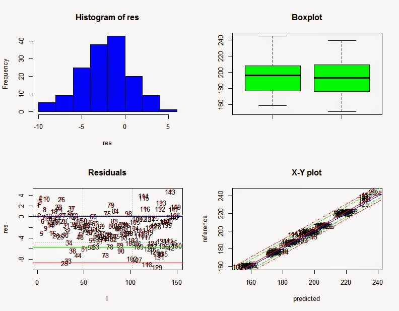
The results show an improvement in the RMSEP and the SEP statistic tell us the error corrected by the bias. The monitor function now recommend a Bias adjustment.

The distribution of the residuals shows the bias problem, but it is quite uniform once we correct the bias.

 

 

------------------------------------- 
N Validation Samples  = 150 
N Calibration Samples = 150 
N Calibration Terms   = 3 
------------------------------------- 
RMSEP    : 3.642 
Bias     : -2.249 
SEP      : 2.875 
UECLs    : 3.327 
***SEP is bellow BCLs (O.K)***
Corr     : 0.9917 
RSQ      : 0.9834 
Slope    : 1.002 
Intercept: 1.874 
RER      : 29.92   Good 
RPD      : 7.759   Very Good 
BCL(+/-): 0.4637 
***Bias adjustment is recommended***
Residual Std Dev is : 2.884 
***Slope adjustment in not necessary***

Monitor function 27-11-2014

Once developed a model with the math treatments we consider adequate, and using the Calibration Samples for Instrument 1 (following with the Shootout_2002 tutorial), the idea is to check if that model performs fine with Instrument 2 for exactly the same samples. A bias is expected, because even being the same model of instrument, differences in the hardware components, optics, alignments,…, apart from some others are the cause of this bias.

Some time ago I develop a function to monitor, to plot and obtain the statistics necessaries to take some decisions as if the bias or slope should be adjusted, to check for outliers of high residuals,.....

 

It is clear that we have 5 outliers of high residuals that the literature about this set considers that must be removed, so the error RMSEP will decrease.
Due to the high RMSEP of the model used for this monitor (RMSEP=4.33 using 4 terms and with all the samples), the bias must be quite high in order to be consider that it should be adjusted. This error is more than 3 times the Lab error.

So the statistics are:

monitor14(monit.tr2[,2],monit.tr2[,1],155,4,0.95,4.33)

Where 0.95 is the confidence interval and 4.33 the CV error of the model using 4 terms

N Validation Samples  = 155 
N Calibration Samples = 155 
N Calibration Terms   = 4 
------------------------------------- 
RMSEP    : 4.942 
Bias     : -2.509 
SEP      : 4.272 
UECLs    : 4.951 
***SEP is bellow BCLs (O.K)***
Corr     : 0.9811 
RSQ      : 0.9626 
Slope    : 0.9813 
Intercept: 6.122 
RER      : 19.9   Fair 
RPD      : 5.146   Good 
BCL(+/-): 0.6778 
***Bias adjustment in not necessary***
Residual Std Dev is : 4.266 
***Slope adjustment in not necessary***

We can see how the SEP (error corrected by the bias) is similar to the error of 

the model, so a bias adjustment will help to transfer the model from instrument 1

to Instrument 2.

I will remove the 5 samples and come back with the results.

Solution for the Regression Coefficients (MLR)

I have use one of the examples of the book "Chemometrics in Excel" to play with Matrix formulas in Excel and calculate the regression coefficients (b0, b1,...). As the book explains there is a formula in Excel to calculate them with just one function.
Of course, the regressors are finally the same.

 

You can see how to run this different operations in Excel in my Youtube Channel

Win ISI 4.7.0.14943 available for downloading

Win ISI 7 is available for downlading, click this link to go to the download page of winisi.com and insert your ID and password to access to this version.

You will get a ZIP file and in it there is a document with the new features, and bugs solved.

If you are not registered, you can do it in the link as well, presing the link of the page itself which says "click here to register".

You can try this version and if you find a bug let us know, as Oscar did with the option in Monitor: "Compare Spectra and Equations".

Overplotting scores for Calibration, Test & Validation sets

 

After calculating the PCA for the Shootout Calibra 1 set, I can see the maps of scores for PC1 vs PC2, PC1 vs PC3, PC2 vs PC3,....

But how can I project other sample sets into this PC space?, and in this case  the Shootout Test 1 and Shootout Valida 1.

The idea is to see if the scores for these Test and Valida Set projected into the PCA space of Calibra 1 are into their cloud space, and all the samples are represented, this way we are not extrapolating.

Win ISI Training Meeting (Fátima - Portugal)

Thanks to the assistants to this training and the great welcome to Portugal.

Diagnostics: Some solvent vapors in the noise spectra

Some days ago, Oscar (a follower of this blog) sent me some estrange diagnostics from his NIR Instrument. It was curious that when I plotted every of the 10 noise spectra test (the final diagnostic result is an average on the ten spectra statistics), the peaks increase more and more and in the same direction (in this case negative), and at the same wavelength, it was like if the NIR was measuring something.

 

 

The way that the NIR perform every noise spectra, is measuring first the background in a ceramic plate, and after scans again the ceramic as a sample. So in the ideal case there is no difference, so we should see something similar to a flat line along cero, but if we zoom the spectra, we start to see the noise due to the instrument hardware, if the background is stable. These noise must be random, without special patterns.

There are cases that some mechanical noise give some noise peaks at certain wavelengths, so we can identify an encoder problem, a filter (order shorter) problem,…

Sometimes stray light goes into the detectors, the lamp,the laboratory temperature, or the detectors temperature, can be also unstable. These and other cases are the cause that we see special signatures in the noise spectra.

So coming back to the Oscar spectra, something seems to be in the air of the laboratory which makes those patters. It was not water vapor signature (as we saw in other cases), it was another thing, and it was obvious because of the smell (similar to ammonia).

The noise spectra shows how it was decreasing, and that date (a little bit later) the noise was fine (random), and the smell as well.

Thanks Oscar for the information

Understanding better Hyperspectral Image Analysis

In my last post I recommended the article :
"Near infrared hyperspectral image analysis using R, Part 5", which appears in the NIR News Vol. 25 No. 7 (November 2014).

In the second part of the tutorial, you can develop an animation to see the spectrum of every pixel in a single line of the bread.
We can see the noise spectra of the background, and the spectra of the different pixels in the line of the bread at a certain Y level .

The animation of the first tutorial is in the post: "Animated visualisation of hyperspectral data using R ".

It is really great to see how, how the scientific community is using R, and we hope to see more articles and papers in the future.

Authors:
Y. Dixit, R. Cama,a C. Sullivan, L. Alvarez Jubetea
School of Food Science & Environmental Health, Dublin Institute of Technology, Cathal Brugha Street, Dublin 1, Ireland
A. Ktenioudakib
Department of Food Chemistry & Technology, Teagasc Food Research Center Ashtown, Ashtown, Dublin 15, Ireland

Animated visualisation of hyperspectral data using R

Very useful article in the last issue of NIR News Vol. 25 No. 7 (November 2014), with an amazing tutorial, about how to develop animated vizualizations of hyperspectral NIR images.
See the second part of the tutorial in the post:"Understanding better Hyperspectral Image Analysis".

Authors:
Y. Dixit, R. Cama,a C. Sullivan, L. Alvarez Jubetea
School of Food Science & Environmental Health, Dublin Institute of Technology, Cathal Brugha Street, Dublin 1, Ireland
A. Ktenioudakib
Department of Food Chemistry & Technology, Teagasc Food Research Center Ashtown, Ashtown, Dublin 15, Ireland

 

 

SG 2nd Derivative + MSC

As you know derivatives remove the baseline offset and curvature in the spectra, but the should be combined with anti-scatter math treatments if we want to remove scatter effects which affect the correlation between the constituents of interest and the spectral bands. There are some cases (especially when developing discriminant models), where it is not convenient to apply the anti-scatter math treatments and we just leave the derivatives alone.

Following the Shoot-out tutorial and following the paper "Shoot-out 2002: transfer of calibration for content of active in a pharmaceutical tablet", from David W. Hopkins (NIR news Vol14 No. 5 2003), I tried the math treatment recommended by the author and apply the MSC after the SG2D1104, just to have a look to the spectra:

You can see how the red spectra, has been calculated in the previous post, and for the green one (SG second derivative combined with MSC), I use the following script:

> X1_sg2dmsc<-msc(X1_sg2d_pracma)
> matplot(wavelength2[11:281],t(X1_sg2dmsc[,11:281]),type="l",
+ xlab="Wavelength (nm)",ylab="1/R (SG 2nd der + MSC)",lty=1,
+ col=3,main="SG-2D1104 + MSC")
If we want to see them over-plotted

Max Kuhn Interviewed by DataScience.LA at useR 2014

Learn more about this great R developer (Caret Package) in this link

Applying SG to all our X matrix (Pracma Package)

"R" is without any doubt a great and wonderful community,  and it is nice to see how the package developers and maintainers help you in case you have any doubts.

It was the case some time ago when was writing some posts about the ChemoSpec package and Bryan Hanson helps me with some doubts. After the last post, I wrote a mail to Hans Werner (Pracma Package) , and he replied quickly, telling me the reason the "savgol" function use a vector indeed a matrix, and giving to me some ideas, to convert all the spectra matrix to Savitzky Golay.

Of course one of the ways is to use the apply function. When applying the SG filters there is  a reduction in the number of data-points at both sides of the wavelengths, depending of the window size.

 So I tried this way, to see all the spectra together:

> library(pracma)
# This script is for first derivative
> X1_sg1d_pracma<-apply(nir.training1$X,1,savgol,11,4,1)
> matplot(wavelength2[11:281],(X1_sg_pracma
+[11:281,]),type="l",xlab="Wavelength (nm)",
+ ylab="1/R (SG 1st derivative)",lty=1,col=1,main="SG-1D1104")

 

# This script is for second derivative
> X1_sg2d_pracma<-apply(nir.training1$X,1,savgol,11,4,2)
> matplot(wavelength2[11:281],(X1_sg_pracma
+[11:281,]),type="l",xlab="Wavelength (nm)",
+ ylab="1/R (SG 2nd derivative)",lty=1,col=1,main="SG-2D1104")

 

Savitzky Golay filters with Pracma Package

Pracma package has the function "savgol", where we can apply Savitzky Golay filter to a vector (in our case a spectrum).
The function is:
  savgol(T, fl, forder, dorder)

And the Arguments are:
 T... Vector of signals to be filtered.
fl... Filter length (for instance fl = 51..151), has to be odd.
forder... Filter order (2 = quadratic filter, 4 = quartic).
dorder... Derivative order (0 = smoothing, 1 = first der, etc.).

As you know I´m using in my last post the shoot-out 2002 data to develop a tutorial, and I read an article from the winner of this shoot-out where he use the shoot-out spectra with Savitzky Golay, a filter of 11, quartic, and second derivative using the Unscrambler software.

So I try thess values in the arguments of the Pracma SG filter and the results of the bands look exactly the same that the ones in the article, so this option looks good to work with this data. Anyway I will try also with the other functions from other packages.

In the case of the Pracma package we have to use a vector (a single spectrum), so some work has to be done to convert all the matrix of spectra, but the results looks great.

X1_sg_pracma<-as.matrix(savgol(nir.training1$X[1,],11,4,2))

PCAs with three diferent methods and projections (Test and Val Set)

The shoot-out 2012 is composed with 155 samples for the training set (Blue color), 460 for the Test Set (Red color), and other few samples for the Validation set (Green color).

I have developed 3 different ways of Principal Components Analysis and I would like to show you the score plot of PC1 vs PC2 developed with the Training Set and the projections on that space of the Test and Validation Set.

This first plot is in the case  of using PRCOMP:

Second case is using NIPALS for the calculation of the PCAs:

and third using SVD for the calculation of the PCAs

As you can see no differences, and we can have the conclussions that the Training Set cover the variability for the samples of the Test Set and Validation Set, so we don´t have to extrapolate outside the calibration space.

I will writte a post with the code (quite long) if interested. Let me know.

 

Adding Category Variables to a Data frame in R

Normally I used data frames to manage NIR data, the data frames are composed normally in my case by a X  or Spectra matrix (dataframe$X), and a Y or constituent matrix (dataframe$Y). But when we want to manage and understand plots, like score plots, it is interesting to classify the samples with some category variables.

This category variables can be: "location", "type", "customer", "product",.....

In the case of the shoot-out data the samples can be classify by their content of the main parameter, and can be classified as:

"Low"             (if the sample has less than 160 mg)
"Medium"          (between 160 y 221 mg)
"High"            (more than 221 mg)

Let´s create the variable in the data frame of the training set for instrument 1
nir.training1$type[Y <=160] <- "Low"
nir.training1$type[Y>160 & Y<221] <- "Medium"
nir.training1$type[Y>=221] <- "High"
Now we have a new variable in the data frame called "type"
Check it with:

names(dataframe)

and appart from X and Y we have Type.

We proceed the same way for the other dataframes.

Another thing is that we can create a big data frame with all the spectra from different instruments and sets and create a category variable for the instrument ( A and B), and another for the Set (Training, Test and Validation).

An introduction to the "´Resamble" package

Some time ago I wrotte a post : An introduction to the "prospectr" package . There I gave a list of some  Chemometric Packages for R. Some days ago in a NIRS forum gave the name of another Chemometric package, so the options to use Chemometrics with R are growing day by day.

This package is "Resamble". This is the link to the reference Manual.

 

More details at:

http://cran.r-project.org/web/packages/resemble/

http://l-ramirez-lopez.github.io/resemble/

The author explains that with this package algorithms such as LOCAL and locally weighted PLS regression can be easily reproduced.
I really want to test it as soon as I can.

Hyperspectral Imaging and Applications Conference 2014

Few days for this interesting Conference, you can see the programme in this link or downladed in PDF here.

NIR Hyperspectral Imaging will be part of the applications conference, for some of the speakers, like Aoife Gowen talk about:

For more details visit the Web Page at: http://www.hsi2014.com/

Adapters from USB to Serial RS232 / RJ45

I have found three kind of connections when installing a NIR to a Computer: Serial Port, USB and RJ45.
 

Now is quite difficult to find a computer with a serial port, so the best option is to connect an adapter from USB to Serial RS232, but I have found that some of them performs fine to all the instruments and software´s, and others give connection problems. The adapters come with the drivers disk

  

USB connections are not a problem, because all the computers have several USB ports.

 

Some new NIR use the Ethernet connection RJ45, and normally all the computers have one, but we need another to connect the computer to a Network and Internet. We can buy a RJ45 board and install it into the computer, but I heard that in some cases is not easy the configuration, so one easy and quick solution is to connect an adapter from USB to RJ45. There are several in the market. They come with the drivers for 32 or 64 bytes.
 

SNV + Detrend with "Prospectr" package

I was using the function “detrend” from the “pracma” package, but we have the detrend function in the “prospectr” package. Using this last option we combine the SNV with the Detrend, which is a very common math-treatment to remove the scatter.

Looking to the function script the “sweep” function is used to center and scale the spectra matrix.

 

Using the shootout 2002 data:

>X1_detrend2<-detrend(nir.training1$X,

+wav=as.numeric(colnames(nir.training1$X)))

>matplot(wavelength2,t(X1_detrend2),type="l",lty=1,

+xlab="Wavelength(nm)",ylab="1/R",col=3,

+main="SNV + Detrend")

I compare with these plots the way prospectr runs the SNV detrend versus the other way I used in other posts.

Green with prospectr package and blue with pracma package.

2nd derivative using "apply" and "diff"

This is a simply exercise, where we convert the raw spectrum into its first derivative, and into its second derivative, using the function apply, and the function diff.

I use the shootout 2002 data available in the package ChemometricsWithR.

X1_diff1<-t(apply(nir.training1$X,1,diff))

In this case the 1 is to apply the function difference to the rows (spectra).

We don´t add more than the default options to the function diff, so the lag=1 and the value of differences=1.

The spectrum changes (losing 1 data point) to the black spectrum in the plot at the end of the post.

plot(as.numeric(colnames(X1_diff1)),X1_diff1 [1,],type="l",xlab="Wavelength (nm)",ylab="1/R (1st derivative)",lty=1,col=1)

We can say briefly that the second derivative is the derivative of the firs derivative; we can do this changing the value of the option “differences” from 1 to 2, losing, in this case two data points.

X1_diff2<-t(apply(nir.training1$X,1,diff,differences=2))

par(new=TRUE)

plot(as.numeric(colnames(X1_diff2)),X1_diff2[1,],type="l",xlab="Wavelength (nm)",ylab="1/R (2nd derivative)",lty=1,col=2)

The spectrum of the second derivative is the red one in the plot, compared with the black one of the first derivative.

This way to do the derivatives is very noisy, so in future post we will try to use gap derivative which is the way that softwares as Unscrambler, Win ISI and many others use the derivatives.