Quitando el scatter con un segundo término en MLR

Regression planes in R (wavelength space)

We have seen the high correlation between wavelengths in previous posts and how we can reduce the wavelength space from lower dimension plots. 

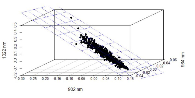
In the case of the 3 wavelengths selected in the previous post at 1022, 964 and 902 nm. 

We can use the wavelength at 1022 nm as the dependent variable and to calculate a MLR regresión to predict the absorbances at this wavelength as a linear combination of the absorbances at 902 and 964 nm calculating a regression plane;
    #1022nm     datapoint 87    
  # 902nm     datapoint 27  
  # 964nm     datapoint 58   
x1<-X_msc_mc[,c(27)]  
x2<-X_msc_mc[,c(58)]  
x3<-X_msc_mc[,c(87)]  
s3d<-scatterplot3d(x1,x2,x3,pch=16,highlight.3d = TRUE,
                   angle=330,xlab="902 nm",
                   ylab="964 nm",zlab="1022 nm")       
fit<-lm(x3~x1+x2)
s3d$plane3d(fit,lty.box = "solid")

We can see the plane looking to the new regression plane plot:

 

x1new=-1.170e-16+(-2.122e+00*x1) 
x2new=-1.170e-16+(-1.061e+00*x2) 
#plot(x1new,x2new)
x12new<-cbind(x1new,x2new)
library(chemometrics)
drawMahal(x12new,center=apply(x12new,2,mean),
          covariance=cov(x12new),quantile=0.975,col="blue")

 

 

Linear combinations to improve correlation

With the data from soy meal on IFT conveyor, I select three wavelengths for this demo:
# 1022nm     datapoint 87     Protein or Oil  
#  902nm     datapoint 27     Cellulose        
#  964nm     datapoint 58     CH2 Oil          
x1<-X_msc_mc[,c(87)]
x2<-X_msc_mc[,c(27)]
x3<-X_msc_mc[,c(58)]

We have the values for Protein for these spectra.

Protein <- Prot

Let´s see the wavelengths in the mean centered MSC treated spectra

matplot(wavelengths,t(X_msc_mc),type="l",
        xlab="wavelengths",ylab="Absorbance")
abline(v=1022)
abline(v=902)
abline(v=964)

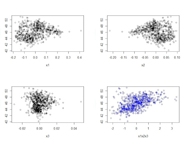
now see how the correlation becomes better in the case of the 4td plot where the X axis is a linear combination of the other 3 wavelengths

 

x1x2x3<-((139.98*x1)+(287.12*x2)+(121.02*x3))

par(mfrow=c(2,2))
plot(x1,Protein)
plot(x2,Protein)
plot(x3,Protein)
plot(x1x2x3,Protein,col="blue")

 

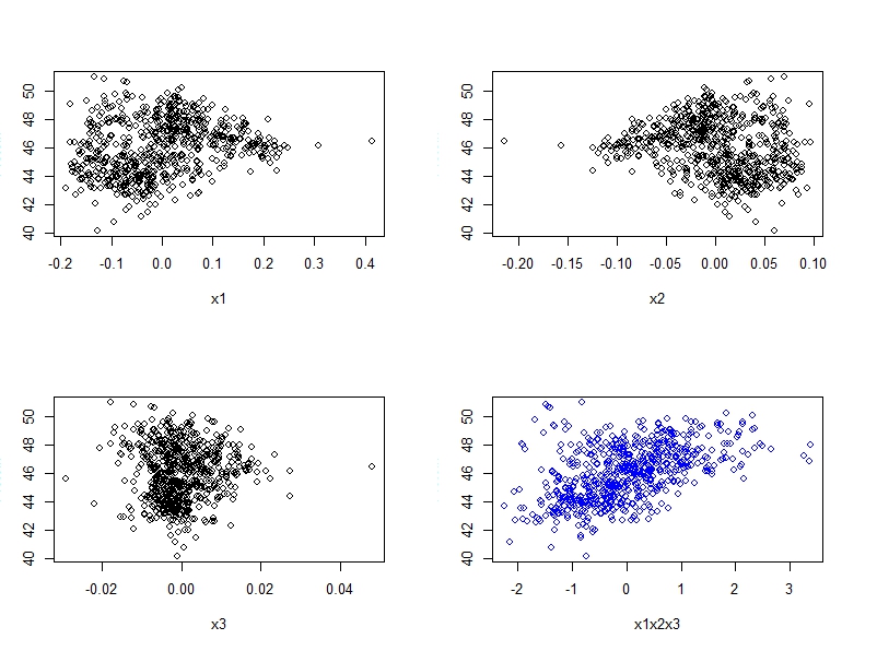
We have worked with this data before with PLS and PCR and what we have done here is a MLR approach. An intercept value will place the date on the same scale.

 

Solution for the Regression Coefficients (MLR)

I have use one of the examples of the book "Chemometrics in Excel" to play with Matrix formulas in Excel and calculate the regression coefficients (b0, b1,...). As the book explains there is a formula in Excel to calculate them with just one function.
Of course, the regressors are finally the same.

 

You can see how to run this different operations in Excel in my Youtube Channel

Step-up & Stepwise Regressions with R

We know that a spectrum has a serial of variables ("x1","x2",....."xm", one at each wavelength), which are the photometric responses for a certain sample. Once we have a certain number of samples "n", we want to develop ‘a model to predict a constituent "y".

Practicing with a table from the book "Introduction to Multivariate Statistical Analysis in Chemometrics" we can set the basis to understand the concepts of "Step-up" and "Stepwise" Regression.

Let´s see the RSQ of each wavelength vs. the "y" variable:

(cor(x1,y1))^2    0.4768583

(cor(x2,y1))^2    0.4112143
(cor(x3,y1))^2    0.02528684

 

 

We can see that  variables "x1" and "x2" have some correlation, but the variable "x3" has a very poor correlation with "y1".

So we start the model with just one term (the x1), and we will add a new term, which will improve the model with a high F test value, we can try with "x2" and "x3", and we clearly see that the model will improve adding "x2" (better XY plot for x1_2 than for x1_3).

 

 

res1_2<-lm(y1~x1+x2)

#Intercept= 1.3528 x1= 4.4328 x2= 4.1164

Improving the RSQ to:

(cor(x1_2,y))^2    0.8880725

 

Adding "x3" to the model as a third term does not improve the RSQ, because it has a very low coefficient (practically cero).

x1_2_3<-1.41833 + 4.42317*x1 + 4.10108*x2 -0.03574*x3 
(cor(x1_2_3,y1))^2   0.8883945

We can use the function step to find the better combination of variables to develop a model. In the case of just 3 , we can proceed as this:
lm_all<-lm(y~x1+x2+x3)
lm_step<-step(lm_all,direction="both")
summary(lm_step)

The summary give us the best variables to use and the regression coeficients: b0, b1 and b2 ( as we can see, with the same results than for "res1_2")
#(Intercept):1.3528 x1= 4.4328 x2= 4.1164

--------------------------------------------------------------------------------------------------------------------------

Let´s use now the package "Chemometrics", with NIR data:

The spectra are:

 

 

 We use the stepwise function from the chemometric package to get values as:

$usedtime

$bic (Bayesian information criterion)

$models
$varnames
RSS (Residual Sum of Squares) is an statistic wich decrease as far as we add a new term, so the BIC formula has a penalty every time we add a new term.

BIC is an statistic which is decreasing as far as we improve the model, variables are added or dropped until the BIC can not be reduced more.

The wavelengths ($varnames) selected are:

"X1115.0" "X1185.0" "X1215.0" "X1385.0" "X1420.0" "X1500.0" "X1565.0" "X1585.0" "X1690.0" "X1715.0" "X1720.0" "X1815.0" "X1995.0" "X2070.0" "X2100.0" "X2195.0"

So we can go ahead with the regression:

y ~ X1115.0 + X1185.0 + X1215.0 + X1385.0 + X1420.0 + X1500.0 +
X1565.0 + X1585.0 + X1690.0 + X1715.0 + X1720.0 + X1815.0 +
X1995.0 + X2070.0 + X2100.0 + X2195.

 

We have found the 15 wavelengths for the model, but now we want to check how it performs, so we need some data for validation in order to calculate the SEP (standard error of prediction) that we expect for future samples predicted with this model.

We are going to do it using the Cross Validation (CV). As you know, with this type of validation, the total sample set is divided in groups, for example four, one group is used for validation and with the other three a MLR regression is made with the 15 wavelengths (X matrix) and the parameter Glucose (Y matrix). The samples which belong to each group are selected randomly. This process will be repeated for a number of times (in this case 100 times), so it seems to be a well mode to validate our model. This type of Cross Validation is called "k-fold cross validation".

This time I prepare a video, to explain the validation regression procedure.

 

 

 

Recomended book in NIR-Quimiometría to follow tutorials:

MLR: Selección manual vs. automática

En este caso se usaron los espectros sin ningún tratamiento, y se desarrollaron dos calibraciones con dos longitudes de onda:

En la primera seleccionamos las longitudes de onda de forma manual, observando el espectro y con ciertos criterios de donde absorbe el analito (índice de hidroxilo). Se selecciono la segunda para eliminar los efectos de offset de linea base por características físicas (obviamente con tratamientos matemáticos antiscatter, estos resultados serían distintos).

En el segundo caso se dejo al software que seleccionara de forma automática las longitudes de onda.

Se dispone de un conjunto de validación de 7 muestras para ver los estadísticos de predicción (SEP) y comparar cual es la mejor opción.

Los estadísticos muestran como mejor opción la manual.
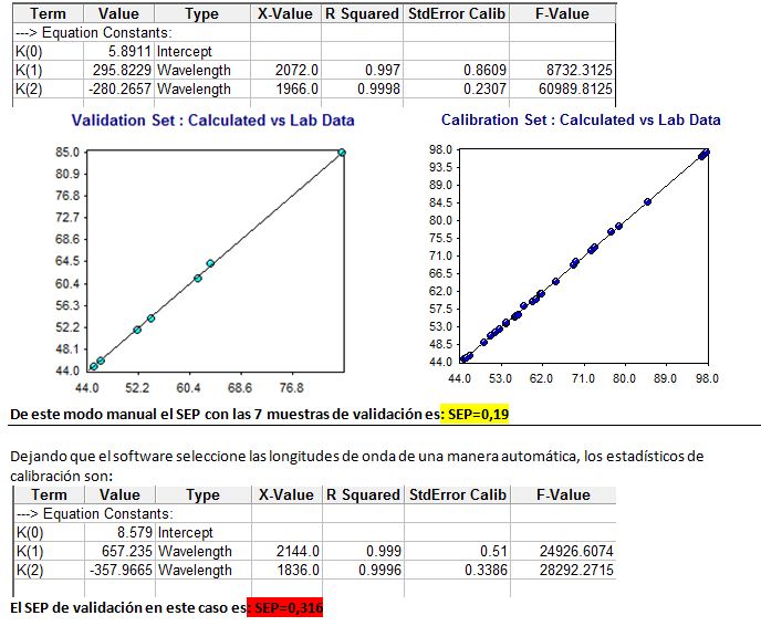
En ambos casos hay una correlación inferior a 0,4 entre las dos longitudes de onda.

MLR: Añadiendo una segunda longitud de onda

Hemos comentado que debemos de intentar seleccionar como primera longitud de onda una que este relacionada con una banda de absorción del analito, de no ser así el software seleccionará la longitud de onda con la mejor correlación con el dato de laboratorio. No obstante debemos comprobar de que sea una correlación directa.

Añadir una segunda longitud de onda se hace para quitar los efectos de interferencia con la primera (algún absorbente que interfiere, efectos debidos a particularidades físicas de la muestra,......). Es por tanto conveniente observar el espectro.

Al añadir la segunda longitud de onda se añade un nuevo coeficiente K(2) y tanto K(0) como K(1) cambian, para conseguir entre los tres la máxima correlación entre el dato de laboratorio y el predicho y por tanto el menor error de calibración.No obstante esto es engañoso, pues a medida que añadamos más términos la correlación aumentará y el SEC bajará. Por tanto debemos de observar ciertas cosas: 

Es importante que las dos longitudes de onda elegidas no estén correlacionadas.

Observar el estadístico F.

Usar un conjunto de validación externo para comprobar la evolución del error de validación.

Karl Norris fue el pionero de estas técnicas de regresión y tiene una increíble sexto sentido para interpretar espectros y seleccionar longitudes de onda y coeficientes por adición, división,....

MLR: Misma Regresión en Vision y Win ISI

Por supuesto obtendremos los mismos resultados que en Excel tanto en Win ISI, Vision, como en Unscrambler, Matlab,... Aquí se aporta también el estadístico F que calculan del mismo modo estos dos software, y del que hablaremos en próximas entradas, así de la complejidad al añadir nuevas longitudes de onda y con ello nuevos coeficientes a la ecuación.

MLR: Regresión en Excel

Tomando los datos de absorción de los espectros (raw spectra) de la entrada anterior a 2072 nm, y los valores de los constituyentes para estos espectros, podemos desarrollar una sencilla regresión simple, calculando los coeficientes de regresión K(0) y K(1) de modo que la predicción de cualquier muestra nueva será:

y = k(0) * k(1)X , siendo X el valor de absorción a 2072 nm para el espectro sin ningún tratamiento.
Las muestras están ordenadas por valor creciente de constituyente.