Tidyverse and Chemometrics (part 14): Extending the database

We have merged the 40 calibration files of  "fish1" and the 17 (of 40) selected samples of "fish2"  so we have a new database with 57 samples and we have to repeat the process we have done in previous posts, in this post creating again the principal components analysis, looking the scores plots, the Mahalaniobis ellipses,....,etc.

We can coloured the scores by their season value, so we can see how every season extend the scores in the different principal components maps.
fish_1d_all_pc<-nipals(fish_1d_all$nir_1d,10)
rownames(fish_1d_all_pc$T)<-fish_1d_all$Sample
colnames(fish_1d_all_pc$T)<-seq(1,10,by=1)
##### Creating a list for NIPALS
library(chemometrics)
fish12_nipals <-list(scores=fish_1d_all_pc$T,
                     loadings=fish_1d_all_pc$P,
                     sdev=apply(fish_1d_all_pc$T, 2, sd))

Now we plot the orthogonal and scores distances and we check which ones are outside  certain limits, coulouring the samples by their season and using 5 principal components.

res<-pcaDiagplot(fish_1d_all$nir_1d,X.pca=fish12_nipals,
                 a=5,col=fish_1d_all$Season)

Samples outside the cutoff are the Mahalanobis distance outliers considering 5 principal components.

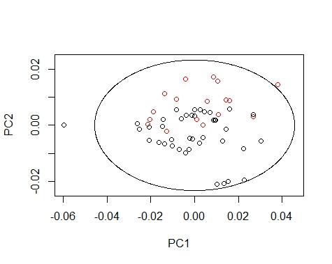
We can draw the Mahalanobis Ellipses with the combinations: PC1 vs PC2,
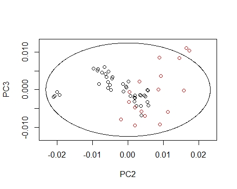
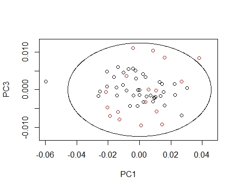
PC1 vs PC3, and PC2 vs PC3. Samples are coloured by their season (black for fish1 and red for fish2). 

library(chemometrics)
par(mfrow=c(1,1))#######  PC2 vs PC3  ##########
 drawMahal(fish_1d_all_pc$T[,c(1,2)],
          center=apply(fish_1d_all_pc$T[,c(1,2)],2,mean),
          covariance=cov(fish_1d_all_pc$T[,c(1,2)]),
          quantile=0.975,xlab="PC1",ylab="PC2",

          col=fish_1d_all$Season)

#######  PC2 vs PC3  ##########
drawMahal(fish_1d_all_pc$T[,c(2,3)],
          center=apply(fish_1d_all_pc$T[,c(2,3)],2,mean),
          covariance=cov(fish_1d_all_pc$T[,c(2,3)]),
          quantile=0.975,xlab="PC2",ylab="PC3",
          col=fish_1d_all$Season)

 

#######  PC1 vs PC3   ########
drawMahal(fish_1d_all_pc$T[,c(1,3)],
          center=apply(fish_1d_all_pc$T[,c(1,3)],2,mean),
          covariance=cov(fish_1d_all_pc$T[,c(1,3)]),
          quantile=0.975,xlab="PC1",ylab="PC3",
          col=fish_1d_all$Season)

Samples out of the ellipse can be identified with the identify function but that does not mean that it is an outlier because that depends of a general computation between all the principal components. 

As you can see all the process is becoming very straightforward as we continue with more posts of more fishing seasons.