PCR vs. PLS (part 5)

It´s time for an external validation with an independent test. Samples in the calibration are from soy meal scanned in a NIT instrument (850 to 1050 nm), but there was some years without testing the calibration with new samples so I have the ocasión to scan new samples in a new instrument (from a new generation). Of course the path-length for transmission must be configure to the same value and the sample must be representative.

 

The validation set has 25 samples were we try to find the wider range as possible. The reference values comes principally from two laboratories, but there are two samples from a different laboratory.

 

we develop in the lasts posts a PCR calibration where we saw that with 10 terms we obtained the better results, but maybe this value is high in order to make the calibration more transferable. The test validation will help us to check this.

 

If we don´t consider the Lab origin, and we over-plot the results of predictions over the XY calibration (including cross validation predictions), we get this plot:

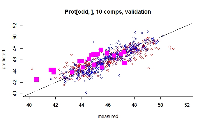
There are some samples that fit quite well, others have a Bias, and other random error. So we want to understand better what is going on, so we can give a color depending of the lab which gives the reference value.

 

plot(pred_pcr_test,Prot_test,xlim=c(40,52),
       ylim=c(40,52),cex=2,pch=21,
     bg=(Lab_test),col=Lab_test,lwd=4,xlab="",ylab="")
plot(pred_pcr_test,Prot_test,xlim=c(40,52),
     ylim=c(40,52),cex=2,pch=21,
     bg=(Lab_test),col=Lab_test,lwd=4,xlab="",ylab="")
legend("topleft",legend=c("Lab1", "Lab2","Lab3"),
       cex=1.5,pch=19,
       col=c(1:3))

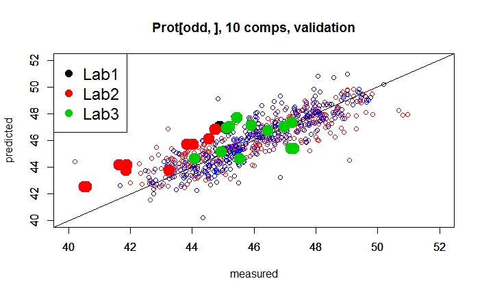
Well, we can take some conclusions from this plot, but we need to check the predictions with different number of terms to see if the Estándar Error of Prediction (with 10 terms the RMSEP is 1,65) decrease and the RSQ (with 10 terms 0,593) increase.