Sunflower seed Regressions with "R" - 001

I have spectra from sunflower seed grinded from 3 NIR instruments (range 400-2500 nm). I prepare the data frame separating the spectral range in two segments (Segment 1 or VIS from 400-1100 nm, and segment 2 or NIR from 1100 to 2500). Reference values are from four different laboratories.
 

In a previous post I have transformed the NIR raw spectra to MSC, using a function from the R package "Chemometrics with R".
 

In this post I want to run a regression with PLS (PLSR) using the Segment 2, and with the math treatment MSC.

sflw1 <- plsr(G00rmn~NIRmsc, ncomp = 10,data =sflw.msc2 ,
        validation = "LOO")

VALIDATION: RMSEP
Cross-validated using 107 leave-one-out segments.
      
          (Intercept)  1 comps  2 comps  3 comps   4 comps   5 comps  6 comps

CV           2.87         2.465       2.074      1.112      1.038     0.9903     0.9833
adjCV      2.87         2.465       2.074      1.111      1.038     0.9899     0.9829

                         7 comps  8 comps  9 comps  10 comps
CV                     0.9746     0.9781    0.9754    0.9683
adjCV                0.9741     0.9775    0.9745    0.9675


 TRAINING: % variance explained

              1 comps  2 comps  3 comps  4 comps  5 comps  6 comps  7 comps  8 comps
X              41.93     89.86       95.78      97.02      98.21      99.21      99.62      99.76
G00rmn    31.47     51.80       86.47      89.14      90.36      90.64      91.01      91.42

              9 comps  10 comps
X              99.81     99.89
G00rmn    92.30     92.62

 

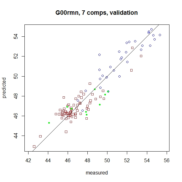
And now we can see the X-Y plot for the LOO Regression (with 7 comps), with different colors and symbols for the samples from the different instruments.

plot(sflw1, ncomp = 7, asp = 1, line = TRUE,

pch=c(20:22)[sflw.msc2$Operator],
col=c("green","blue","brown")[sflw.msc2$Operator])