Tidyverse and Chemometrics (part 14): Extending the database

We have merged the 40 calibration files of  "fish1" and the 17 (of 40) selected samples of "fish2"  so we have a new database with 57 samples and we have to repeat the process we have done in previous posts, in this post creating again the principal components analysis, looking the scores plots, the Mahalaniobis ellipses,....,etc.

We can coloured the scores by their season value, so we can see how every season extend the scores in the different principal components maps.
fish_1d_all_pc<-nipals(fish_1d_all$nir_1d,10)
rownames(fish_1d_all_pc$T)<-fish_1d_all$Sample
colnames(fish_1d_all_pc$T)<-seq(1,10,by=1)
##### Creating a list for NIPALS
library(chemometrics)
fish12_nipals <-list(scores=fish_1d_all_pc$T,
                     loadings=fish_1d_all_pc$P,
                     sdev=apply(fish_1d_all_pc$T, 2, sd))

Now we plot the orthogonal and scores distances and we check which ones are outside  certain limits, coulouring the samples by their season and using 5 principal components.

res<-pcaDiagplot(fish_1d_all$nir_1d,X.pca=fish12_nipals,
                 a=5,col=fish_1d_all$Season)

Samples outside the cutoff are the Mahalanobis distance outliers considering 5 principal components.

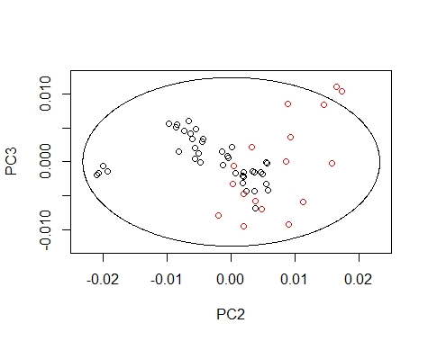
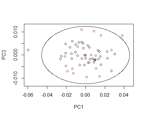
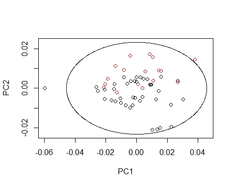
We can draw the Mahalanobis Ellipses with the combinations: PC1 vs PC2,
PC1 vs PC3, and PC2 vs PC3. Samples are coloured by their season (black for fish1 and red for fish2). 

library(chemometrics)
par(mfrow=c(1,1))#######  PC2 vs PC3  ##########
 drawMahal(fish_1d_all_pc$T[,c(1,2)],
          center=apply(fish_1d_all_pc$T[,c(1,2)],2,mean),
          covariance=cov(fish_1d_all_pc$T[,c(1,2)]),
          quantile=0.975,xlab="PC1",ylab="PC2",

          col=fish_1d_all$Season)

#######  PC2 vs PC3  ##########
drawMahal(fish_1d_all_pc$T[,c(2,3)],
          center=apply(fish_1d_all_pc$T[,c(2,3)],2,mean),
          covariance=cov(fish_1d_all_pc$T[,c(2,3)]),
          quantile=0.975,xlab="PC2",ylab="PC3",
          col=fish_1d_all$Season)

 

#######  PC1 vs PC3   ########
drawMahal(fish_1d_all_pc$T[,c(1,3)],
          center=apply(fish_1d_all_pc$T[,c(1,3)],2,mean),
          covariance=cov(fish_1d_all_pc$T[,c(1,3)]),
          quantile=0.975,xlab="PC1",ylab="PC3",
          col=fish_1d_all$Season)

Samples out of the ellipse can be identified with the identify function but that does not mean that it is an outlier because that depends of a general computation between all the principal components. 

As you can see all the process is becoming very straightforward as we continue with more posts of more fishing seasons.

Present and Future of R-Studio (2020 conference talks)

                              
                               

Tidyverse and Chemometrics (Part 13): Monitoring Fish2 predictions

Now that we have the 17 selected samples with the lab values, it is time to process their spectra through the model to see their predictions and to compare the predicted and reference values to compare them and get a serial of statistics, which will tell us if the model is performing adequately.

In the histograms we have seen that the model should extrapolate in some way to predict the extension of range that some fish2 selected samples are requiring. We know that 40 samples are not a great number of samples but it can be used as starter calibration that we will improve as we add more samples with a structure procedure, selecting the samples that increase the model´s variability so we reduce the number of samples to send to the laboratory.

To predict the samples we need them converted with the mat treatment used for the samples which participate in the model (the 40 samples of Fish1), after that in the case of the PLS model we use the function "predict" to get the results for the four constituents: "Dry Matter", "Protein", "Fat" and "Ash".

 

fish2_pls_prot_pred<-predict(fish1_prot_plsr,

                     ncomp = 8,

                     newdata = fish2_sel_df$nir_1d)
fish2_pls_dm_pred<-predict(fish1_DM_plsr,

                     ncomp = 3,

                     newdata = fish2_sel_df$nir_1d)
fish2_pls_fat_pred<-predict(fish1_FAT_plsr,

                      ncomp = 4,

                      newdata = fish2_sel_df$nir_1d)
fish2_pls_ash_pred<-predict(fish1_ASH_plsr,

                      ncomp = 9,

                      newdata = fish2_sel_df$nir_1d)

 

Now we create a table with four columns of predictions

 

fish2_sel_pred<-cbind(fish2_pls_dm_pred,

                fish2_pls_prot_pred,

                fish2_pls_fat_pred,

                fish2_pls_ash_pred)

 

and merge it with the data frame which contains the sample numbers and laboratory reference values for these samples.

 

fish2_selected_monitor<-cbind(fish2_selected,fish2_sel_pred)

 

Now we can use the Monitor package to study the statistics. The Monitor package is not an available package by the moment. I have been developing this package and at the moment I am writing the documentation to see if it can be accepted by R, if this it is not possible I will load it on GitHub for people interested on it.

 

The Monitor package apart of many statistics create a serial of plots, I I include in this case the XY plots for the predictions of the 17 samples of Fish2 with the Fish1 Model. As expected we have a Bias which indicates that the model it is not robust yet, but the SEP (error corrected for the bias) it is quite good. The idea is that we have 57 samples to develop a new calibration and we will find another future validation set to test it.

 

library(Monitor)
# For Dry Matter
monitor_xyplot(fish2_selected_monitor[,c(1,4,8)])

#For Protein
monitor_xyplot(fish2_selected_monitor[,c(1,5,9)])

#For Fat
monitor_xyplot(fish2_selected_monitor[,c(1,6,10)])

#For Ash
monitor_xyplot(fish2_selected_monitor[,c(1,7,11)])

 

 

 

Tidyverse and Chemometrics (part 12): Comparing histograms Fish1 and Fish2

Well, finally lab values for the selected samples are here and it is time to see if we have expanded the calibration set used with the Fish1 season with the selected samples from the new Fish2 season. One way to do it it is comparing the histograms of the 40 samples of Fish1 and the 17 selected from Fish2 (from the total 40 available).

Let´s start with the "Protein":

library(tidyverse)
ggplot(fish_1d_all,aes(PROTEIN)) +
    geom_histogram(data=subset(fish_1d_all,Season == "Fish1"),
                                fill = "blue", alpha = 0.2) +
    geom_histogram(data=subset(fish_1d_all,Season == "Fish2"),
                                fill = "red", alpha = 0.2)

As you see I merge the 40 samples of Fish1 and the 17 of Fish2 and a column factor to indicate the season. So the Fish 2 samples for expansion are in red and the 40 of Fish 1 in blue, and the result is:

There is a high expansion in the range of "Protein", let´s see for the other parameters:

High expansion for "Ash", and not so large but also useful for "Fat" and "Dry Matter". Now it´s time to see how the model developed with the 40 Fish1 samples predict the 17 Fish2. But this will be in the next post.

Convertir ficheros ".nir" en ".cal" importando de Excel

Tidyverse and Chemometrics (part 11): Removing redundant samples

We have seen in the last post, how the fish2 spectra was projected on the principal component space designed by the fish1 spectra. We saw clearly than some of the fish2 samples were out of the ellipse and others were in, but not very close to the fish1 samples. At the same time, some samples of fish2 are neighnors between them or some probably are neighbors of fish1 samples.

We can measure the distance from one sample to another by the Mahalanobis distance. We use to call this distance “Mahalanobis Neighborhood Distance”, and depending of the threshold we use around each sample, more or less samples are selected as neighbors.

The first I want to do is to remove neighbors in fish2, in order to select a percentage (50% approx.) of the fish2 samples to send to the lab for reference analysis. With this intention, I use the function “puchwein” from “prospecr” package and I note the selected samples to make a “fish2_selected” file. In this case, “puchwain” creates a new PC space with the fish2 samples and measure the distance between their scores. With this configuration the selection are 21 samples, so 19 are redundant.

 

pchw_fish2<-puchwein(nir_fish2_2d,pc=0.95,k=0.2,

                     min.sel=20,details=TRUE,

                     .center = TRUE,.scale = FALSE)

Now we have to check if the selected samples have neighbours into the samples of fish1, so we use fDiss from prospect to compare the distances between the scores of fish1 and the scores we got with the projections of the 21 selected samples on the PC space of fish1. If we set a threshold of 0.2 we see that four of the selected samples have neighbors on fish 1 (positions 5, 13, 19 and 20), so we remove them from the selected set, so finally we have 19 samples to send to the laboratory.

 

summary(fDiss(Xr=nir2d_pc$T[,1:5],

             X2=fish2_2d_T_sel1[,1:5],

             method = "mahalanobis",

             center = TRUE, scaled = FALSE))
neig_f2f1<-fish2_2d_T_sel1[c(5,13,19,20),]
fish2_2d_T_sel2<-fish2_2d_T_sel1[-c(5,13,19,20),]

Once we have done it, we can overplot again all the samples:

• Fish1 samples in blue.
• Fish2 redundant samples in red.
• Fish2 selected samples in green
• Fish2 neighbors of Fish1 in orange.

Now we wait for the laboratory values, ….,see you in the next post.

Tidyverse and Chemometrics (part 11): Proyecting Fish2 on Fish1 PCs

Once I have the PCs for the 40 fish meal samples calculated on the previous post is time to project the new samples on the fish1 PCs in order to see which samples will fill and expand the space.

 

First we have to calculate the fish2 scores on the fish1 principal components space multiplying the X matrix of fish1 by the loadings matrix "P" of fish1 PCs, and the results are the scores of fish2 on fish1 PCs.

 

Now if we use the drawMahal from the Chemometrics Package we get these plots which show that we need to send some of the fish2 samples to the lab to expand the calibration.

As we can see samples goes apart specially on the third PC. What you think can be the reason?.

PC1 is quite related to moisture and it does seem that this constituent is not two much expanded with fish2 spectra, but which constituent is specially represented by the third loading of the fish1 PCs loadings?.