Tidyverse and Chemometrics (part 9)

The idea of these "tidyverse and chemometrics" tutorials is to create enough code to prepare a training about chemometrics with R and to follow the rules I commonly use when I develop a calibration with other chemometric softwares. In the previous post we have seen how we have 40 samples of fish meal and we want to use them to create a starter calibration with the idea to increase the number of samples in the future spending the less money as possible in laboratory data.

As the tutorials go through I will sometimes come back to previous steps if necessary, trying to find the best configuration as possible to the models math treatments and predictions.

In the previous model we developed the calibration with Caret, and this time we will do it with the PLS package, with the same math treatments SNV+DT+First Derivative.

So the code to create the new dataframe  we are goings to use is:

library(prospectr)
nir_snvdt<-detrend(nir,wavelength)

once the snv+dt is applied we apply the first derivative

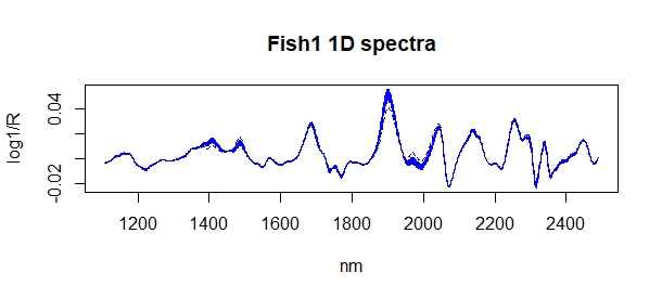
nir_1d<-gapDer(nir_snv,m=1,w=1,s=4)

the first derivative truncate the spectra on the extremes, so the range change:

wavelength_1d<-seq(1108,2490,2)        #new range for the 1D
matplot(wavelength_1d,t(nir_1d),type="l",col="blue",
        xlab="nm",ylab = "log1/R",
        main="Fish1 1D spectra")

Sample ID and constituent values are the same whichever the math treatment is:

 

fish1_1d_df1<-data.frame(sample_id,month,year,dm,

                         protein,fat,ash,I(nir_1d),

                         stringsAsFactors = FALSE)

 

Now we can develop the PLS model using the Leave One Out Cross Validation option:

 

library(pls)

fish1_prot_plsr<-plsr(protein~nir_1d,data=fish1_1d_df1,

validation="LOO",ncomp=10)

 

Now we will create a first plot that will help us to take the decisión of how many terms to use for the model:

 

par(mfrow=c(1,2))
plot(fish1_prot_plsr,"validation", estimate="CV")

 

with the number of terms with the lowest RMSE (8), we create the XY plot for predicted vs reference values:

 

par(pty="s")
plot(fish1_prot_plsr,"prediction",ncomp=8)

 

 

 

 As you can see we get the same results than the regression win Catet in the previous post.