Eye on Agriculture Today: Soil Texture By Feel

Nice video which explains how to determine soil texture by feel:

PCA with the first derivative

In a previous post we had calculated the PCA with the math treatment SNV+Detrend and we calculated a first sample set of outliers with the Mahalanobis distance. 

When calculating PCA we have to treat as best the spectra as possible in order to detect populations or boundaries and if we treat the spectra with math treatments which help to do this task is great. So indeed, to apply the SNV + Detrend, I apply this time the first derivative to the spectra (soil from Spanish soil from LUCAS database) and calculate the PCA.

We can have a look to the score’s maps (six PC recommended) to find if there are boundaries on them:

Look at the maps which include PC2 as one of the axes. There are a certain number of samples which takes a different direction than the rest. This second PC term can be useful to find something interesting on the spectra.

 To see what is happening we can see the loading spectra for this second PC term:

This loading spectra has the first derivative math treatment applied, so we can compare it with a library of reference known spectra (minerals in this case) to see which is the best match, and in this case the best match is with the gypsum mineral, so this second term is explaining part of the variance included in our spectra database due to the addition of gypsum to the soil.

LUCAS SP Database vs. pure mineral Gypsum

In order to find if the soil has traces of a certain mineral, it is useful to overplot our soil samples (in this case the soil Spanish samples included in the LUCAS database, with the pure mineral spectrum  (in this case Gypsum). We must  overplot them with the same math treatment and in the same scale. I do it, in this case, with the spectra treated with the SG second derivative.

 In red is the pure gypsum mineral and in grey samples in the soil database.  As we can see some of the bands match, so we can be quite sure that there are some samples in the database with gypsum content to certain levels.

Second derivative is quite helpfull to find these matches. If we do it, for example with SNV+Detrend, some of the bands are hiden by other samples and the assumption that there are samples with gypsum is less clear.

Detecting outliers with Mahalanobis distance

In this first plot we see the spectra of the LUCAS spanish database treated with the SNV and Detrend math treatment of the "Prospectr" package, where we remove the quadratic trend (as we saw in the last post):

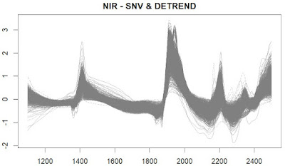
The next step is to calculate the Principal Components Analysis, where we calculate the scores of every sample for the selected components. These scores are stored in a score matrix, which have a centre.

The next step is to measure the distance from every sample projected in the PC space to this centre. This distance (calculated with the function "fdiss" from the "resamble" package) can be represented in a plot aconsidering the spectra with distances higher than 3.00 as outliers.

Which are this samples? just mark them on the first plot and take out some conclusions:

As we can see they seem to be quite different of the average spectrum (considered the center), but we can consider that there are other samples which are not selected as outliers and they seem to be. 

The normal procedure is to remove in a first step these samples, and calculate again the new centre with the rest and proceed with a new mahalanobis distance calculation

Quadratic trendlines

In the last post, I talk about the use of the function "detrend" in the package "prospectr" to remove the quadratic trend lines in the soil NIR spectra. We can see these trendlines overplotted to the spectra (I do it just for five of the soil spectra from the Spanish soil LUCAS database).

In red is the spectra treated with SNV and in blue the quadratic trend lines to apply to the SNV treated spectra, to remove them and convert them in a SNV + Detrend spectra.