Detecting outliers with Mahalanobis distance

In this first plot we see the spectra of the LUCAS spanish database treated with the SNV and Detrend math treatment of the "Prospectr" package, where we remove the quadratic trend (as we saw in the last post):

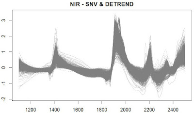
The next step is to calculate the Principal Components Analysis, where we calculate the scores of every sample for the selected components. These scores are stored in a score matrix, which have a centre.

The next step is to measure the distance from every sample projected in the PC space to this centre. This distance (calculated with the function "fdiss" from the "resamble" package) can be represented in a plot aconsidering the spectra with distances higher than 3.00 as outliers.

Which are this samples? just mark them on the first plot and take out some conclusions:

As we can see they seem to be quite different of the average spectrum (considered the center), but we can consider that there are other samples which are not selected as outliers and they seem to be. 

The normal procedure is to remove in a first step these samples, and calculate again the new centre with the rest and proceed with a new mahalanobis distance calculation

Quadratic trendlines

In the last post, I talk about the use of the function "detrend" in the package "prospectr" to remove the quadratic trend lines in the soil NIR spectra. We can see these trendlines overplotted to the spectra (I do it just for five of the soil spectra from the Spanish soil LUCAS database).

In red is the spectra treated with SNV and in blue the quadratic trend lines to apply to the SNV treated spectra, to remove them and convert them in a SNV + Detrend spectra.

Scale and linear / Scale and quadratic

Scale and linear and Scale and quadratic are two of the scatter corrections that we can find in Win ISI 4, and they are used to remove as much as possible the multiplicative scatter we found in the NIR spectra. Two are the packages that have a detrend function in R, so depending on the case of the multiplicative effect (linear or quadratic, we can use the pracma or prospectr packages.

The detrend function of the Prospectr package is equivalent to the math treatment in WinISI 4 called "scale and quadratic” and combine the SNV treatment with the remove of a quadratic trendline in the spectra. In the case of the combination of SNV and Detrend from the Pracma package we obtain the Win ISI math treatment "Scale and Linear" and in this case we remove the linear trend line due to the scatter. We can try both to check which one gives the better performance.

I show the spectra of both treatments applied to the soil LUCAS database spectra filtered for the Spanish soils:

Samples are coloured according the soil type (cropland, grassland, woodland,....). The jump in the detector change it is common due that we treat individually the math treatment for the NIR and VIS ranges (trend are different in VIS and NIR regions).

Trim spectra from LUCAS database

The spectra from LUCAS database (ESDAC*) seem to come from a XDS  (VIS + NIR) instrument, and this instrument give two options when exporting the spectra (every 0.5 nm, and every 2 nm), the data comes in 0.5 nm, and that means that we have 4200  data poits per spectrum, and that means a huge spectra matrix.

We can trim the spectra keeping just the spectral data every two nanometers, so we will have the reflectance values from 400 to 2498 nm every 2nm, so we have a less heavy matrix of 1050 data points per spectrum. This fuction will give us the spectra like a NIR6500.

Just create a sequence to select one column of every four, and call that function (like in my case) "trim05to2":

dim(lucas_spain$spc)
 2604 4200

spec2nm <- trim05to2(lucas_spain$spc)

dim(spec2nm)
 2604 1050

*European Soil Data Centre (ESDAC), esdac.jrc.ec.europa.eu, European Commission, Joint Research Centre

Importing LUCAS database from R into WinISI

Once we have the spectra we want from the LUCAS database (ESDAC*) in R, we can export it to a "txt" file with:


write.table(spec2nm, file="lucas_spain.txt",
            row.names=TRUE,
            col.names=FALSE)

This way we have the samples IDs, but we don´t need the column name (wavelengths), because Win ISI will create them when importing the spectra.

Once we have the txt file, we convert it to a ".nir" file which is the spectra format for Win ISI with the Win ISI tool "Convert", selecting the configuration from TXT to Win ISI.

After filling  the options Win ISI ask, we wait for the conversion succeeded message and we have the ".nir" file ready to view:

Now we do the same with the parameters (constituents) we are interested in:

write.table(lucas_spain[ ,c(1, 5:16)],                                           file="lucas_spain_constituents.txt", 

            row.names=TRUE, col.names=TRUE)

We export the samples IDs as well, to link them with the spectra. Finally we import the parameters to the spectra to get the ".cal" file and ready to work with the spanish LUCAS database in Win ISI.

*European Soil Data Centre (ESDAC), esdac.jrc.ec.europa.eu, European Commission, Joint Research Centre