Tidyverse & Chemometrics (Part 1)

Along this year, I am going to write a number of posts to work with R and Near Infrared spectra using the "tidyverse" package (and also others), so this will be a way I will learn how to use it.

 

So let´s start with some fish meal data (40 samples) acquired during a certain fishing season , so this will be our starter database and we will updated and validated using spectra of new samples from  other seasons.

 

The constituents are Moisture, Protein, Fat and Ash, and they are in a data frame with other columns as the Sample ID, Month, Year and of course the absorbances at a certain range (from 1100 to 2448 nm).

 

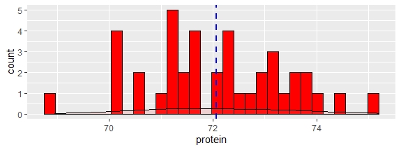
The name of the data frame is "fish1_df", and the first thing I do is to get the histograms to check the distributions for the parameters:

library(tidyverse)
#for the Dry Matter:
fish1_df %>%
ggplot(aes(dm))+
  geom_histogram(fill="blue",col="black")+
  geom_density(alpha=.2, fill="#FF6666") +
  geom_vline(aes(xintercept=mean(dm, na.rm=T)),
               color="red", linetype="dashed", size=1)

 

fish1_df %>%
ggplot(aes(protein))+
  geom_histogram(fill="red",col="black")+
  geom_density(alpha=.2, fill="#FF6666") +
  geom_vline(aes(xintercept=mean(protein, na.rm=T)),
               color="blue", linetype="dashed", size=1)

 

ggplot(aes(fat))+
  geom_histogram(fill="green",col="black")+
  geom_density(alpha=.2, fill="#FF6666") +
  geom_vline(aes(xintercept=mean(fat, na.rm=T)),
               color="blue", linetype="dashed", size=1)

fish1_df %>%
ggplot(aes(ash))+
  geom_histogram(fill="brown",col="black")+
  geom_density(alpha=.2, fill="#FF6666") +
  geom_vline(aes(xintercept=mean(ash, na.rm=T)),
               color="red", linetype="dashed", size=1)