An introduction to the "prospectr" package

prospectr: An interesting package that we will use to apply to our tutorials and data. I like that it has an algorithm (SELECT) used in Win ISI and the name of the function is "shenkWest" (Shenk and Westerhaus, develop the SELECT algorithm for Win ISI), so we have more tools to use R in spectroscopy.

Don´t forget that we have also other packages like:

ChemoSpec

hyperSpec

cluster

mvoutlier

pls

signal

soil.spec

caret

...
You will find  PDF tutorials for these packages on the Web, and for others like ChemometricsWithR and chemometrics, there are even some books.

 

Comparing regressions with different scatter math-treatments (Shootout 2002 Tutorial)

In a previous post, we have developed the calibration without any math-treatment with the Training Set from Instrument 1, without any treatment , knowing that it was not the best choice, and we look to the LOO (leave one out) cross validation errors to check the performance.

Now we develop the regressions with some anti-scatter math-treatments to compare the cross validation errors and to decide which of them performs better. Anyway the shootout supplies also a test set, so validating with this test set will give us a better idea about how the calibration is performing with independent data.

 

First thing to do is to convert the “X1. Training” and “X1. Test” matrix to the math treatment we want to use: SNV (Standard Normal Variate), Detrend , SNV + Detrend and MSC.

>nir.train1_snv<-data.frame(X= I(X1_snv),Y=I(Y))

>nir.train1_detrend<-data.frame(X= I(t(X1_detrend)),Y=I(Y))

>nir.train1_snvdt<-data.frame(X= I(t(X1_snvdt)),Y=I(Y))

>nir.train1_msc<-data.frame(X= I(X1_msc),Y=I(Y))

Now we can develop the PLS regressions:

 

>mod1_snv<-plsr(Y~X,data=nir.train1_snv,+

 ncomp=10,validation="LOO")

>mod1_detrend<-plsr (Y~X,data=nir.train1_detrend,+

 ncomp=10,validation="LOO")

>mod1_snvdt<-plsr(Y~X,data=nir.train1_snvdt,+

 ncomp=10,validation="LOO")

>mod1_msc<-plsr(Y~X,data=nir.train1_msc,+

 ncomp=10,validation="LOO")

We can plot the RMSEP values versus the number of components (or terms), to have a better idea of the performance of the models (black line is the model without mat-treatments or raw spectra, green line is with just Detrend, the rest (SNV, SNV+DT and MSC) are almost overlaped.

 

But if we want to see it with more details, we have to see the numbers provided by the summary of the models. I mark in yellow the smallest values.

 

 

But the question can be: Do we have to choose the number of components which gives the small RMSEP?.

We will reply to this question soon.

In a next post we will do the same with derivative mixed with scatter corrections to see if we get better values for RMSEP and we will check it with an external validation (don´t forget that these RMSEP are for Cross Validation).

 

 

 

 

 

 

SNV and Detrend (Shootout 2002 NIR with R)

I want to say “thanks” to Aoife Gowen (@eefieg) for the references, in her last article to this blog. The article is the part 4 of a series called “NIR hyperspectral image analysis using R” and the title of this article is: "Pretreatments and partial least square discriminant analysis". (NIR News Vol.25 Nº 5 August 2014).
 

Lately I am playing with the Shootout 2002 data so we can summarize on this data things that we have seen before in the blog.
 

In the last post, I was using the raw spectra and that is not (in some cases) the best way to develop a calibration. So we treat the raw spectra with math treatments to improve the correlation of the spectra with the reference values, and to make more transferable calibrations. If we use a correct math-treatment the regressions will use less terms, and will improve the statistics, and the transferability.

Now I write the script used to treat the matrix X1 (training spectra matrix in Instrument 1):

>par(mfrow=c(2,2),ps=14)
>matplot(indices,t(nir.training1$X),type="l",col=1,

 + main="Raw Spectra")
#Applying "SNV" to the Shootout 2012 Data>X1_snv<-scale(t(nir.training1$X),center=TRUE,scale=TRUE)
>matplot(wavelength2,X1_snv,type="l",

 + xlab="Wavelength (nm)",ylab="1/R",lty=1,

 + col=2,main="SNV math_treat")
#Applying "Detrend" to the Shootout 2012 Data

>library(pracma)
>X1_detrend<-detrend(t(nir.training1$X))  
 +matplot(wavelength2,X1_detrend,type="l",

 +lty=1,xlab="Wavelength(nm)",ylab="1/R",col=3,

 +main="Detrend math_treat")
#Combining SNV with Detrend

>X1_snvdt<-detrend(X1_snv,tt="linear")

>matplot(wavelength2,X1_snvdt,type="l",lty=1,

 +xlab="Wavelength(nm)",ylab="1/R",col=4,

 +main=" SNV+Detrend math-treat")

 

As we are writing this script, we see on the Active Graphics Window the spectra , so we can compare them.

These are some of the most familiar anti-scatter math-treatments, apart from others like MSC.

 

We will continue with this type of exercises in the next posts.

XY Plot to compare predictions (same model / diferent instruments)

As we mention several times, plots help us to understand better what is happening. In the previous posts we are working with the shootout 2002 data in order to work with as many tools as possible we have in R to understand this data set and to make a model we can use to predict as better as possible a validation set.
Plotting the predictions of the Test set acquired in Instrument 2 with the model developed with the Training set of samples acquired in Instrument 1, versus the predictions of the test set acquired in instrument 1, can give us an idea that there is something more than a simple bias, and that we have to take into account a group of samples that behaves differently.
Lets see that plot:
1) We make the predictions of the Test1 set with Model 1 and stored it in:
  anl_tst1_mod1<-predict(mod1,ncomp=3,
+ newdata=data.frame(Y=I(Y.test),X=I(X1.test)))
2) We make the predictions of the Test2 set with Model 1 and stored it in:
  anl_tst2_mod1<-predict(mod1,ncomp=3,
+ newdata=data.frame(Y=I(Y.test),X=I(X2.test)))
3) Now we plot the predictions versus reference for anl_tst1_mod1
  plot(Y.test,anl_tst1_mod1,col="blue",ylim=c(150,240))
4) Now we write the script:
   par(new=TRUE)
5) Now we plot the predictions versus reference for anl_tst2_mod1
  plot(Y.test,anl_tst2_mod1,col="red",ylim=c(150,240))
6) Now we get this plot:

We can see that most of the samples behave similarly with a bias

 

If interested to follow this tutorial see also:

Working with the Shootout 2002 (NIR) in R

Plotting the predictions (Working with the Shootout 2012 NIR data in R)

Comparing Spectra and Coefficients (Shootout 2002 NIR with R)

 

 

 

Comparing Spectra and Coefficients (Shootout 2002 NIR with R)

We can check the differences between the instruments 1 and 2 more in different ways. One could be to select 5 samples, and compare their spectra scanned in Instrument 1 and scanned in instrument 2. In this case I select from the training set samples 10,20,30,40 and 50.
The samples look like this:

But the best to see the differences, is to substract the spectra, so I made some substractions:
dif1<-selected[1,]-selected[6,]
dif2<-selected[2,]-selected[7,]
dif3<-selected[3,]-selected[8,]
dif4<-selected[4,]-selected[9,]
dif5<-selected[5,]-selected[10,]
and combined them:
dif<-rbind(dif1,dif2,dif3,dif4,dif5)
Now we can see the spectra of the differences (quite similar for the 5):

 

 

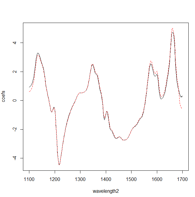
When developing the models (mod 1 and mod 2), we obtain the regression coefficient, which are like a spectra, so we can compare them:

 

 

and also substract them:

 

to obtain some conclussions.

 

 

 

 

 

Plotting the predictions (Working with the Shootout 2012 NIR data in R)

This post follows the previous one: "Working with the Shootout 2012 (NIR) in R".
We have predicted the Test file scanned in Instrument 2 with the model developed with the Training file scanned in Instrument 1 (mod 1), and we have seen that the RMSEP is higher than the RMSEP obtained predicting the Test file scanned in Instrument 1 with the same model mod1. The X-Y plot will give us a better idea of what is going on.
This figure represents the predictions of the Test Set scanned in instrument 1 with the model mod1:
predplot(mod1,ncomp=3,newdata=data.frame(Y=I(Y.test),X=I(X1.test)),
asp=1,line=TRUE)

The next figure represents the predictions of the Test Set scanned in instrument 2 with the model mod1:

predplot(mod1,ncomp=3,newdata=data.frame(Y=I(Y.test),X=I(X2.test)),

asp=1,line=TRUE)

We can see that part of the RMSEP error is due to an important bias, and an increase of the random noise.

This shootout is probably the most famous so there is quite enough articles and documents and as far as we continue with this tutorial, we can see the results compared with other approaches.

 

 

Working with the Shootout 2002 (NIR) in R

I was practicing with the shootout 2002, where you have a certain number of training samples (155), scanned in two instruments 1 and 2, so we have two "Training files" with the same LAB values, but different spectra (due that the samples are acquired in diferent instruments). The idea of the shootout is to develop a robust calibration for both instruments.

So I had  developed a PLS Model in R with the Training samples acquired in "Instrument 1". I called the model "mod1":

mod1<-plsr(Y~X1,data=nir.training1,ncomp=5,validation="LOO").

Where "nir.training1" is a data frame:

nir.training1<-data.frame(X= I(X1),Y=I(Y))

X: is the 155 row training matrix of spectra acquired in Instrument 1

Y: is the reference training matrix of the constituent of interest and this matrix is the same for the Instrument 2, where their matrix of spectra would be X2.

 

after checking the summary of the model I decide that 3 terms (components) are enough for the model.

 

Now  I want to predict the samples of  a Test file (also scanned in 1). This Test file has more samples  (460), so the rows are higher for the Y matrix and for the X matrix. The idea is to get a RMSEP statistic.

RMSEP(mod1,estimate="test",ncomp=3,intercept=FALSE,

+ newdata=data.frame(Y=I(Y.test),X=I(X1.test)))

 

 and I have found several problems getting errors like this:

"newdata' had 460 rows but variables found have 155 rows"

"Error en model.frame.default(formula(object), data = newdata) :

variable lengths differ (found for 'X1')".

I was making some mistakes assigning names to the matrix in the data frame, and they must be the same in both cases (The dataframe from which I develop the regression and the dataframe which I want to evaluate.

nir.training1<-data.frame(X= I(X1),Y=I(Y))

newdata=data.frame(Y=I(Y.test),X=I(X1.test)))

 

Finally I got a value of 4.974 for the RMSEP.

Now the following exercise must be to check if I have a similar error with a calibration develop with a model developed with the Training spectra of Instrument 2 with the Test Set spectra from Instrument 2 (don´t forget that the Y reference values are the same that for instrument 1, because we are using the same samples):
mod2<-plsr(Y~X,data=nir.training2,ncomp=5,validation="LOO")
Three terms are also enough, and the RMSEP for the Test Set scanned in Instrument 2 with the model 2 is:
RMSEP(mod2,estimate="test",ncomp=3,intercept=FALSE,
+ newdata=data.frame(Y=I(Y.test),X=I(X2.test)))

 and the value is: 5,315.

But what would be the RMSEP for the Test set scanned in Instrument 2 and predicted with the model developed with the Training Samples scanned in instriment 1 (mod1):
RMSEP(mod1,estimate="test",ncomp=3,intercept=FALSE,
+ newdata=data.frame(Y=I(Y.test),X=I(X2.test)))

 The result is: 9,983
So the model can not be transfered without doing anything from instrument 1 to Instrument 2, if what we want is to get similar performance in both.
We will continue with this in the next post.