Introduction to the dplyr R package

PCR vs. PLS (part 3)

A common way to develop the regressions with PCR or PLS is with "Cross Validation", where we divide the training data set into groups that you can select depending of the number of samples: In the case you have few samples you can select a high (10 for example) value and in the case you have a lot of samples, you can select a low value (for example 4). One group is keep out and the regression is developed with all the others. We use the group keep outside to validate repeating the process as many times as validation groups.
 

So Iin the case of 4 groups), we obtain 4 validation statistic values as RMSEP, RSQ, Bias,... for every group we use in the development of the regression, so we can see from which term the RMSEP start to become higher, or the RMSEP values are almost flat and make not sense to add more terms to the regression.

 

Really the cross validation help us to avoid over-fitting, but it helps also to detect outliers (good or bad outliers we can say).

 

It is interesting that the samples in the training set have a certain way of sorting or randomnes . We don´t want that there are similar samples in the training and validation set, but this require inspection of the spectra previous to the development of the regression looking for neighbors, or other sources of redundancy. In the case there are similar samples we want that they stay if possible in the same  group.

 

In the development of the PCR, we van select the Cross Validation option and also the number of segments or groups for validation, in this case 10:

Xodd_pcr3<-pcr(Prot[odd,] ~ X_msc[odd,],validation="CV",
           segments=10,ncomp=30)
plot(Xodd_pcr3,"validation",estimate="CV")

If we see the plot of the RMSEP for the 30 terms, we see that the in the fourth the RMSEP decrease dramatically, but after 10 it does make not sense to use those terms, so we have to select 10 or less.

An external validation (if possible with more independent samples) can help us with the decision.

 

A particular case of Cross Validation is the Leave One Out validation, where a sample unique sample is keep out for validation and the rest stay for the calibration. The process is repeated until all the samples have been part of the validation process. So in this case there are the same numbers of segments or groups than number of samples. This process is quite interesting when we have few samples in the training set.

About the X-Y plots (Predicted vs Reference values), it is important to interpret them in the case of cross validation. There are plots which show the predicted values vs the reference values when all the samples are part of the regression (blue dots) and those plots are not realistic, so it is better to see the plot, when every dot (sample), has a value when it is not part of the model because it is  in the validation set (red dots), this way we have a better idea of the performance of the regression for future samples.

 

plot(Xodd_pcr3,"validation",estimate="CV")
plot(Xodd_pcr3,"prediction",ncomp=10,col="red",
     xlim=c(40,52),ylim=c(40,52))
Xodd_pcr3.pred<-predict(Xodd_pcr3,ncomp=10,

                newdata=X_msc[odd,],
                xlab="Predicted",ylab="Reference")
par(new=TRUE)
plot(Xodd_pcr3.pred,Prot[odd,],col="blue",
     xlim=c(40,52),ylim=c(40,52),
     xlab="",ylab="")
abline(0,1)

This is not a nice tutorial set where the samples fit well, but it is what you often fine in several applications where you want to try to get the best model for a certain product parameter and instrument.

eRum 2018 (European R users meeting)

The European R Users Meeting, eRum, is an international conference that aims at integrating users of the R language living in Europe. Although the useR! conference series also serve similar goals, but as it's alternating between Europe and USA (and more recently Australia in 2018), we decided to start another conference series in the years when the useR! is outside of Europe.
Follow @erum2018 

To consider when validating with LOCAL

I talk in other posts about LOCAL calibration. Once the LOCAL model is placed for routine, and the time pass, is time for validation.

 

LOCAL may have several products merged in a unique database from which we have developed the calibration, so it is important to label every sample in the validation set with a value (in this case 1: Black, 2:Red and 3:Green) corresponding to 3 different types of pork meat meal.

 

The validation is just to compare the reference values from the laboratory and the predicted values from our Near Infrared Instrument in this case, and the best way to represent it is a XY plot. The constituents most important in meat meal are: Moisture, Protein, Fat and Ash.

 

A first look to the general XY plots will gives an idea how it works:

The plot tell us that we have to split the validation set into 3 validation sets one for every class to calculate the statistics for every one.
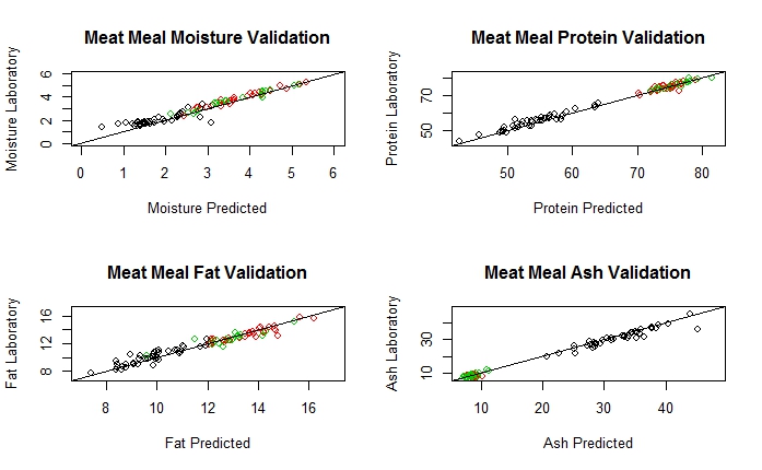
In the case of Protein we will get this validation:

For the Green product:

For the Red Product:

For the Black Product:

As we can see we have a significant Bias for product 1, but not for the other two products, so we can proceed with the validation adjustments (3 products linked to a LOCAL database, and one of them bias adjusted until the calibration is updated).

 

Plots with R

 

 

PCR vs. PLS (part 2)

Continue from post: "PCR vs PLS (part 1)":

As we add more terms to the model (PCR or PLS) the Standard Error of Calibration decrease and decrease, for this reason is necessary to have a validation method to decide how many terms to keep.

Cross Validation, or an External Validation set are some of the options to use.

The "PLS" R package has the function "RMSEP" which give us the standard error of the calibration, and we can have an idea of which terms are important for the calibration.

Continuing with the post PCR vs PLS (part 1), one we have the model we can check the Standard Error of Calibration with the 5 terms used in the model.

RMSEP(Xodd_pcr, estimate="train")
(Intercept)      1 comps      2 comps      3 comps      4 comps      5 comps  
      1.985        1.946        1.827        1.783        1.167        1.120 

 

As we can see the error decrease all time, so we can be tempted to use 5 or even more terms in the model.

One of the values of the  pcr function is "fitted.values" which is an array with the predictions depending of the number of terms.

As we can see in the RMSEP values, 4 seems to be a good number to choose, because there is a big jump in the RMSEP from R PC term 3 to PC term 4 (1.783 to 1.167), so we can keep the predicted values with this number of terms and compare it with the reference values to calculate other statistics.

 

Anyway these statistics must be considered as optimistic and we have to wait for the validation statistics (50% of the samples in the even position taken apart in the post "Splitting Samples into a Calibration and a Validation sets" .

Statistics with the Odd samples (the ones used to develop the calibration)
pred_pcr_tr<-Xodd_pcr2$fitted.values[,,4]
##The reference values are:
ref_pcr_tr<-Prot[odd,]
## We create a table with the sample number,
## reference and predicted values
pred_vs_ref_tr<-cbind(Sample[odd,],ref_pcr_tr,pred_pcr_tr)

Now using the Monitor function I have developed:
monitor10c24xyplot(pred_vs_ref_tr)

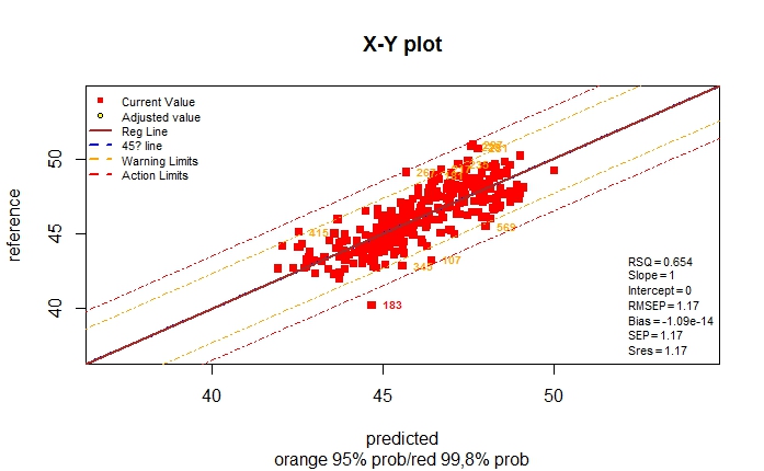
We can see other statistics as the RSQ ,Bias,...,etc.

Now we make the evaluation with the "Even" samples taken apart for the validation:

library(pls)
pred_pcr_val<-as.numeric(predict(Xodd_pcr2,ncomp=4,newdata=X_msc_val))
pred_pcr_val<-round(pred_pcr_val,2)
pred_vs_ref_val<-data.frame(Sample=I(Sample[even]),
                 Reference=I(Prot_val),
                 Prediction=I(pred_pcr_val))
pred_vs_ref_val[is.na(pred_vs_ref_val)] <- 0  
                 #change NA by 0 for Monitor function

As we can see in this case the RMSEP is a Validation statistic, so it can be considered as the Standard Error of Validation, and its value it´s almost the same as the RMSEP for Calibration.

RMSEP Calibration .........1,17

RMSEP for Validation .....1,13