Plotting NIR spectra with ggplot2

This is the post number two of the Soil spectroscopy training material. We are following the paper Soil spectroscopy training material and at the same time we make small changes to the code.

In the previous post, we plot the NIR spectra using the classical R function matplot. Now we want to use the ggplot2 package to plot the spectra but for that we have to prepare the data in a different way, creating a long format indeed a wide format.

library(tidyverse)
load("dat.RData")
load("C:/BLOG/Workspaces/NIR Soil Tutorial/post1.RData")
#converting the wavelengths into numeric values
my_wavelengths <- as.numeric(colnames(dat$spc_raw))

#creating the long dataframe
vnir_long <- data.frame(
sample = rep(1:nrow(dat), each = ncol(dat$spc_raw)),
oc = rep(dat$Organic_Carbon, each = ncol(dat$spc_raw)),
clay = rep(dat$Clay, each = ncol(dat$spc_raw)),
silt = rep(dat$Silt, each = ncol(dat$spc_raw)),
sand = rep(dat$Sand, each = ncol(dat$spc_raw)),
wavelength = rep(my_wavelengths, nrow(dat)),
absorbance = as.vector(t(log(1 / dat$spc_raw, 10))))

head(vnir_long)

  sample        oc     clay silt sand wavelength absorbance
1      1 0.7950426 14.95713 40.1 44.9        350   1.206405
2      1 0.7950426 14.95713 40.1 44.9        351   1.204785
3      1 0.7950426 14.95713 40.1 44.9        352   1.225360
4      1 0.7950426 14.95713 40.1 44.9        353   1.239876
5      1 0.7950426 14.95713 40.1 44.9        354   1.238837
6      1 0.7950426 14.95713 40.1 44.9        355   1.235567

We can use the ggplot function to create a plot.

ggplot(vnir_long,
aes(x = wavelength, y = absorbance, group = sample, color = clay)) +
geom_line(alpha = 0.5) + # Set alpha to 0.5 for transparency
scale_color_gradient(low = 'blue', high = 'red') +
theme_minimal() +
  labs(x = 'Wavelength (nm)',y = 'Calculated absorbance',color = 'Clay (%)')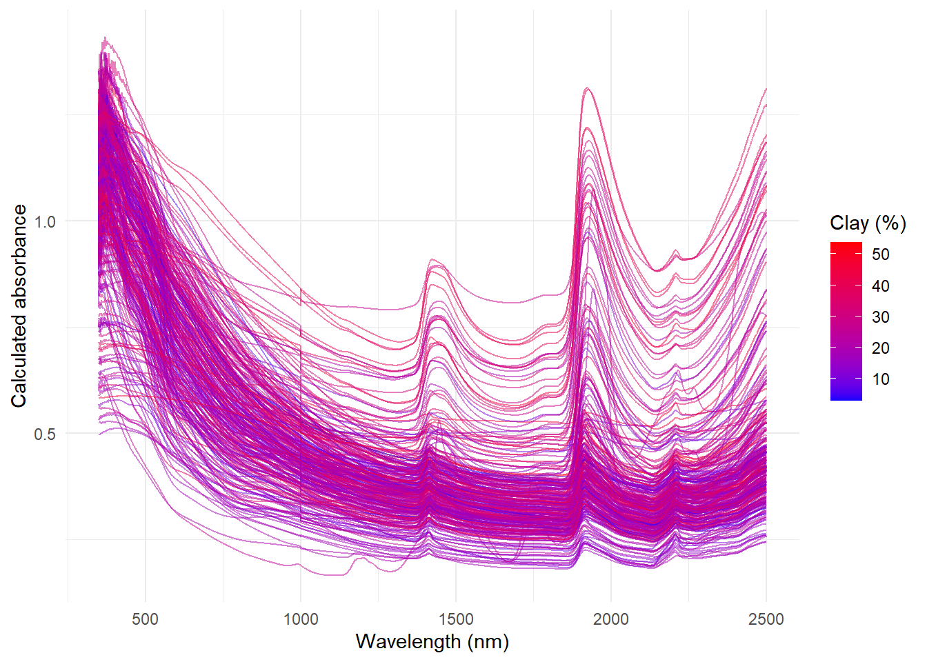

This plot shows the spectra of the samples with the clay content as a color gradient (the paper use the organic carbon). The x-axis represents the wavelength in nano-meters, and the y-axis represents the calculated absorbance. The color gradient indicates the clay content, with blue representing the samples with the lower clay content and the red ones with the higher clay content.

Due to the scatter we don´t see any patters clearly in the spectra yet.

The paper also show us how to work with the MIR (Middle Infrared Spectra), so in the next post we will do the same as we did in these first two posts, but with the MIR dataframe.

Bibliography:

Soil spectroscopy training material Wadoux, A., Ramirez-Lopez, L., Ge, Y., Barra, I. & Peng, Y. 2025. A course on applied data analytics for soil analysis with infrared spectroscopy – Soil spectroscopy training manual 2. Rome, FAO.