Looking for artifacts in the spectra

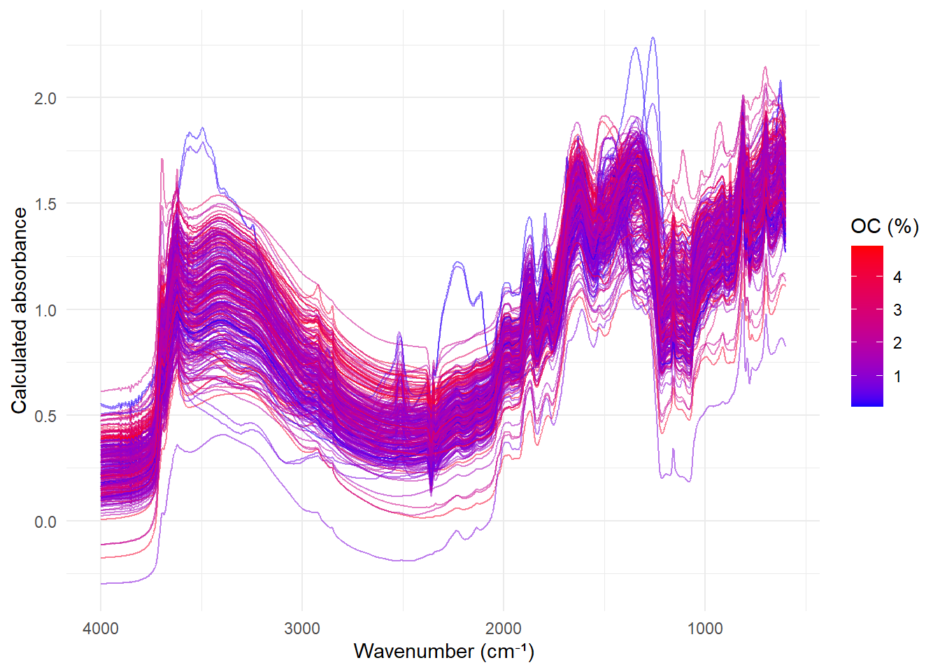
 In this post we are going to look to the NIR spectra in detail looking for artifacts in the sample:

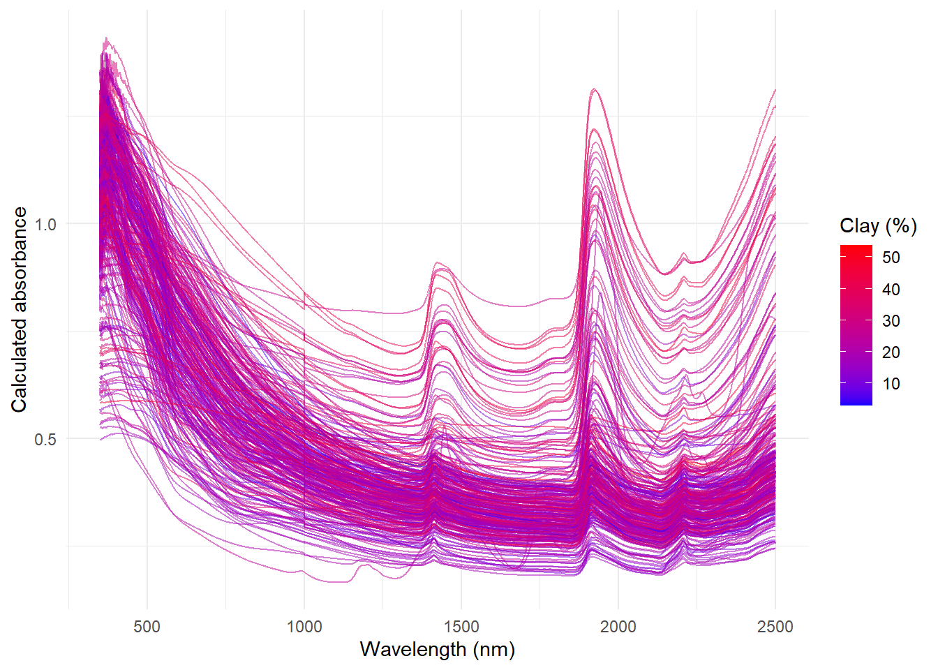
Plotting the spectra :

Looking to the NIR spectra we can see that there are some artifacts in the spectra at 1000 nm and 1830 nm. These artifacts are due to the change of detector in the spectrometer. We can plot these artifacts using the ggplot2 package.

In this case we are going to vave the plots and use the patchwork package to combine them.

library(tidyverse)
library(patchwork)
load("C:/BLOG/Workspaces/NIR Soil Tutorial/post2.RData")

artifact_1000nm <- ggplot(vnir_long,
       aes(x = wavelength, y = absorbance, group = sample)) +
  geom_line(alpha = 0.5) +
  theme_minimal() +
  labs(
    title = "Artifacts at 1000 nm",
    subtitle = "Due to detector change",
    x = 'Wavelength (nm)',
    y = 'Calculated absorbance'
  ) +
  coord_cartesian(xlim = c(990, 1010), ylim = c(0.4, 0.45)) +
  geom_vline(xintercept = 1000, linetype = "dashed", color = "red")

artifact_1830nm <- ggplot(vnir_long,
       aes(x = wavelength, y = absorbance, group = sample)) +
  geom_line(alpha = 0.5) +
  theme_minimal() +
  labs(
    title = "Artifacts at 1830 nm",
    subtitle = "Less visible than at 1000 nm",
    x = 'Wavelength (nm)',
    y = 'Calculated absorbance'
  ) +
  coord_cartesian(xlim = c(1820, 1840), ylim = c(0.2, 0.4)) +
  geom_vline(xintercept = 1830, linetype = "dashed", color = "red")

Combining the plots

We can combine both plots:

artifact_1000nm + artifact_1830nm + plot_layout(ncol = 2)

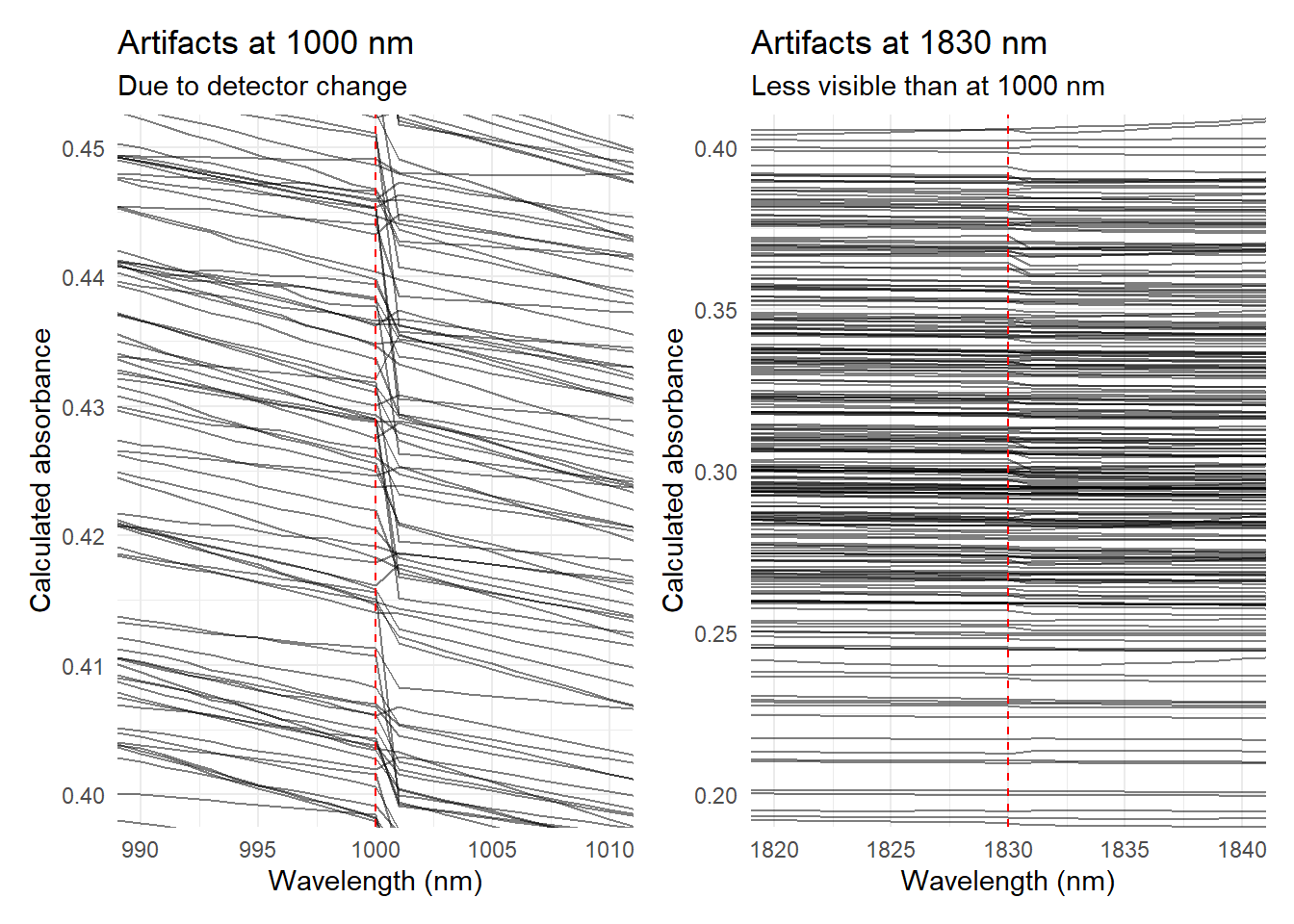
Bibliography:

Soil spectroscopy training material Wadoux, A., Ramirez-Lopez, L., Ge, Y., Barra, I. & Peng, Y. 2025. A course on applied data analytics for soil analysis with infrared spectroscopy – Soil spectroscopy training manual 2. Rome, FAO.

Follow the posts on Netlify

Plotting MIR spectra with ggplot2

 

Loading and preparing the MIR data.

The data is available in the data folder of the repository. Is in a CSV format and can be loaded using the read_csv function from the readr package.

library(readr)

url_mir <- "https://raw.githubusercontent.com/FAO-SID/SoilFER-Spec/main/data/dat2MIR.csv"
dat2MIR <- read_csv(url_mir)

Now we will follow the instructions of the Soil spectroscopy training material changing the name of the first column (index of the samples) to “sample”.

colnames(dat2MIR)[1] <- "sample"
head(dat2MIR, c(10, 7))

# A tibble: 10 × 7
   sample `4001.65608` `3999.72758` `3997.79907` `3995.87056` `3993.94205`
    <dbl>        <dbl>        <dbl>        <dbl>        <dbl>        <dbl>
 1      1       0.180        0.18         0.180        0.180        0.181 
 2      2       0.150        0.151        0.151        0.151        0.151 
 3      3       0.0484       0.0487       0.0489       0.0491       0.0492
 4      4       0.133        0.133        0.133        0.134        0.134 
 5      5       0.227        0.228        0.228        0.228        0.228 
 6      6       0.120        0.120        0.121        0.121        0.121 
 7      7       0.312        0.313        0.313        0.313        0.314 
 8      8       0.225        0.226        0.226        0.226        0.227 
 9      9       0.218        0.219        0.220        0.220        0.221 
10     10       0.113        0.113        0.114        0.114        0.114 
# ℹ 1 more variable: `3992.01354` <dbl>

Looking to the CSV file, we see that the first column is the sample number, and the last one the organic carbon parameter. All the columns in the middle ate the wavenumbers.

Let´s create a vector with the wavenumbers. The wavenumbers are in the column names from the second to the penultimate column, so we can extract them using the following code:

wavenumbers <- as.numeric(colnames(dat2MIR)[2:(ncol(dat2MIR) - 1)])

Let´s prepare the wavenumbers vector to be used as column names in the matrix of spectra.

wavelengths_ir <- round(10000000 / wavenumbers)
wavenumbers_ir <- round(10000000/wavelengths_ir) # Convert to cm-1

my_spectra_ir <- as.matrix(dat2MIR[, 2:(ncol(dat2MIR) - 1)])
colnames(my_spectra_ir) <- wavenumbers_ir

Let´s prepare the MIR dataframe to work with it:

dat_mir <- dat2MIR[, c(1, 1767)]
dat_mir$spc_raw_ir <- my_spectra_ir
rm(my_spectra_ir)

library(tidyverse)

my_wavenumbers <- as.numeric(colnames(dat_mir$spc_raw_ir))

#creating the long dataframe
ir_long <- data.frame(
sample = rep(1:nrow(dat_mir), each = ncol(dat_mir$spc_raw_ir)),
oc = rep(dat_mir$Organic_Carbon, each = ncol(dat_mir$spc_raw_ir)),
wavenumber = rep(my_wavenumbers, nrow(dat_mir)),
absorbance = as.vector(t(dat_mir$spc_raw_ir))
)

head(ir_long)

  sample        oc wavenumber absorbance
1      1 0.7950426       4002    0.17972
2      1 0.7950426       4000    0.18000
3      1 0.7950426       3998    0.18025
4      1 0.7950426       3995    0.18048
5      1 0.7950426       3994    0.18076
6      1 0.7950426       3992    0.18107

We can use the ggplot function to create a plot.

ggplot(ir_long,
       aes(x = wavenumber, y = absorbance, group = sample, color = oc)) +
  geom_line(alpha = 0.5) +
  scale_color_gradient(low = 'blue', high = 'red') +
  scale_x_reverse() +  # Invierte el eje X
  theme_minimal() +
  labs(x = 'Wavenumber (cm⁻¹)',
       y = 'Calculated absorbance',
       color = 'OC (%)')

Bibliography:

Soil spectroscopy training material Wadoux, A., Ramirez-Lopez, L., Ge, Y., Barra, I. & Peng, Y. 2025. A course on applied data analytics for soil analysis with infrared spectroscopy – Soil spectroscopy training manual 2. Rome, FAO.

Follow the NIR-Chemometrics blog on Netlify

Plotting NIR spectra with ggplot2

This is the post number two of the Soil spectroscopy training material. We are following the paper Soil spectroscopy training material and at the same time we make small changes to the code.

In the previous post, we plot the NIR spectra using the classical R function matplot. Now we want to use the ggplot2 package to plot the spectra but for that we have to prepare the data in a different way, creating a long format indeed a wide format.

library(tidyverse)
load("dat.RData")
load("C:/BLOG/Workspaces/NIR Soil Tutorial/post1.RData")
#converting the wavelengths into numeric values
my_wavelengths <- as.numeric(colnames(dat$spc_raw))

#creating the long dataframe
vnir_long <- data.frame(
sample = rep(1:nrow(dat), each = ncol(dat$spc_raw)),
oc = rep(dat$Organic_Carbon, each = ncol(dat$spc_raw)),
clay = rep(dat$Clay, each = ncol(dat$spc_raw)),
silt = rep(dat$Silt, each = ncol(dat$spc_raw)),
sand = rep(dat$Sand, each = ncol(dat$spc_raw)),
wavelength = rep(my_wavelengths, nrow(dat)),
absorbance = as.vector(t(log(1 / dat$spc_raw, 10))))

head(vnir_long)

  sample        oc     clay silt sand wavelength absorbance
1      1 0.7950426 14.95713 40.1 44.9        350   1.206405
2      1 0.7950426 14.95713 40.1 44.9        351   1.204785
3      1 0.7950426 14.95713 40.1 44.9        352   1.225360
4      1 0.7950426 14.95713 40.1 44.9        353   1.239876
5      1 0.7950426 14.95713 40.1 44.9        354   1.238837
6      1 0.7950426 14.95713 40.1 44.9        355   1.235567

We can use the ggplot function to create a plot.

ggplot(vnir_long,
aes(x = wavelength, y = absorbance, group = sample, color = clay)) +
geom_line(alpha = 0.5) + # Set alpha to 0.5 for transparency
scale_color_gradient(low = 'blue', high = 'red') +
theme_minimal() +
  labs(x = 'Wavelength (nm)',y = 'Calculated absorbance',color = 'Clay (%)')

This plot shows the spectra of the samples with the clay content as a color gradient (the paper use the organic carbon). The x-axis represents the wavelength in nano-meters, and the y-axis represents the calculated absorbance. The color gradient indicates the clay content, with blue representing the samples with the lower clay content and the red ones with the higher clay content.

Due to the scatter we don´t see any patters clearly in the spectra yet.

The paper also show us how to work with the MIR (Middle Infrared Spectra), so in the next post we will do the same as we did in these first two posts, but with the MIR dataframe.

Bibliography:

Soil spectroscopy training material Wadoux, A., Ramirez-Lopez, L., Ge, Y., Barra, I. & Peng, Y. 2025. A course on applied data analytics for soil analysis with infrared spectroscopy – Soil spectroscopy training manual 2. Rome, FAO.