Working with Soilspec data (part 8)

We continue in this post with the "chemometrics" package used in the previous one. Indeed the ellipses here we see the cutoff and the samples which are bellow and over it. 

Apart from the graphics we can have a list with the sample number and the robust or classical Mahalanobis distances values.

Is it interesting to see the distribution of the Mahalanobis distances, and for that we can use the histograms:

hist(res$md)    (classical Mahalanobis distance)
hist(res$rd)    (robust distance)

Normally we see the classical histogram in the software we commonly use, due that they use the classical Mahalanobis distance.

Now it is time to reduce the database to take the structure of it, this way can serve to us to send the selected samples to the lab and to save money in the development of the calibration and at the same time keep the variability of the samples. There are several algorithms to do it with the “prospectr” package, being one of then the ShenkWest (nice to have this algorithm in R, and all that workm with Win ISI know it quite well), but I am going to use the “puchwein”, because it seems to me that it capture the structure quite well.

pu <- puchwein(X = PC_scores, k = 0.1, pc =5) 

plot(pu$pc[,c(1,2)], col = rgb(0, 0, 0, 0.3), 

     pch = 19, main = "puchwein")
grid()
points(pu$pc[pu$model,],col = "red", pch = 19) 

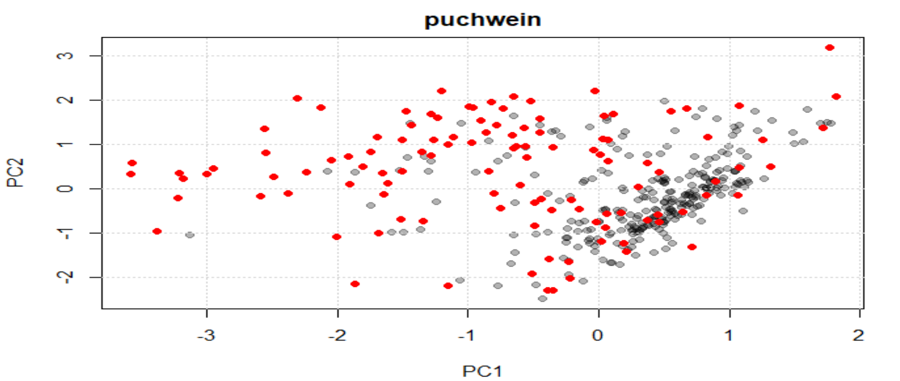
Now we can see the selected samples in the scores map PC1 vs PC2 in red color. These samples keep the structure quite well and can be used to send them to the lab.