Working with Soilspec data (part 11)

Now, I show the plots with main statistics I get with the data I have been using in the previous posts, but don`t forget they are obtained with a simple math treatment like SNV combined with Detrend and with PLS models. In the next posts we will see if we get an improvement using derivatives or some other algorithms apart from the PLS.

There are cases, like the Total Carbon, where we can see some non linearity, than we can maybe handle with ANN, using logs, or some other methods, but in this case we have not enough samples to develop an ANN model, so we will see.

There are some parameters like "Sand" where the performance is poor, but we will see if using derivatives could be improved.

Sure we can get improvements in Clay, Silt and Total Carbon, due that we have a good range. 

Working with Soilspec data (part 10)

 Now it is time for regressions and prediction for all the parameters using the selected spectra with the "puchwain"  function, and for test, the non selected ones.

We develop the regressions with Caret using PLS and Cross Validation (the model choose 5 terms).

model_clay_snvdt <- train(y_sel_clay ~.,data=trainDataClay,  

                          method = "pls", scale = TRUE,

                          trControl = trainControl("cv", number = 10),

                          tuneLength = 20)

We can plot the predictions of the Training Set (selected samples) with the predictions of the Test Set (non selected Samples) for every parameter. I do in this case for Clay :

Working with Soilspec data (part 9)

Once we split the soilspec data into the selected samples (pu$model) and the others (samples non selected  pu$test), we can take them apart with our favorite math treatment (in this case SNV and Detrend):

pu_sel<- spectra_snvdt[pu$model,]
pu_nonsel<- spectra_snvdt[ pu$test,]
matplot(as.numeric(colnames(pu_sel)),t(pu_sel),type = "l",
        col = "blue", xlab = "wavelength", 

        ylab = "Log 1/R")
par(new=TRUE)
matplot(as.numeric(colnames(pu_nonsel)), t(pu_nonsel), 

        type = "l",
        col = "red", xlab = " ", ylab = " ")

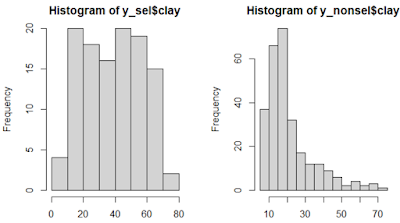
We can do the same for the "Y" matrix with the parameters, and look to one of the histograms (for clay for example):

y_sel<- parameters[pu$model, ]

y_nonsel<- parameters[pu$test, ]

par(mfrow = c(1,2))

hist(y_sel$clay)

hist(y_nonsel$clay)

Now we have a group of samples (the selected ones) to develop the regressions, and we will use the non selected for validation.

Working with Soilspec data (part 8)

We continue in this post with the "chemometrics" package used in the previous one. Indeed the ellipses here we see the cutoff and the samples which are bellow and over it. 

Apart from the graphics we can have a list with the sample number and the robust or classical Mahalanobis distances values.

Is it interesting to see the distribution of the Mahalanobis distances, and for that we can use the histograms:

hist(res$md)    (classical Mahalanobis distance)
hist(res$rd)    (robust distance)

Normally we see the classical histogram in the software we commonly use, due that they use the classical Mahalanobis distance.

Now it is time to reduce the database to take the structure of it, this way can serve to us to send the selected samples to the lab and to save money in the development of the calibration and at the same time keep the variability of the samples. There are several algorithms to do it with the “prospectr” package, being one of then the ShenkWest (nice to have this algorithm in R, and all that workm with Win ISI know it quite well), but I am going to use the “puchwein”, because it seems to me that it capture the structure quite well.

pu <- puchwein(X = PC_scores, k = 0.1, pc =5) 

plot(pu$pc[,c(1,2)], col = rgb(0, 0, 0, 0.3), 

     pch = 19, main = "puchwein")
grid()
points(pu$pc[pu$model,],col = "red", pch = 19) 

Now we can see the selected samples in the scores map PC1 vs PC2 in red color. These samples keep the structure quite well and can be used to send them to the lab.

Working with Soilspec data (part 7)

 Once we have calculated the scores matrix (PC_scores) we can draw the scores maps, and over them the Mahalanobis distance ellipses. 

We must be cautious about this, because we can do it in the classical or robust way and that depends of how we calculate the Covariance matrix. In this case I use the "chemometric" package and compare both. Look at the difference, which is quite large.

Clearly the robust one find the grouping of samples and detects as outliers the rest. Is this really what we want?.

We have to check that group characteristics and see if it would be necessary to create a group apart or to remove redundant samples in that group to give more weight to the rest of the samples, so the ellipse will change.

drawMahal(PC_scores[,c(1,2)],
          center=apply(PC_scores[,c(1,2)],2,mean),
          covariance= cov(PC_scores[,c(1,2)]),
          quantile =0.975)
drawMahal(PC_scores,
          T_mcd$center,
          covariance= T_mcd$cov,
          quantile =0.975)

Working with Soilspec data (part 6)

 Let´s work with the principal components analysis (PCA) with the "datsoilspc" spectra with the math treatment SNV and Detrend. This time we use the Caret package:

library(caret)

spc_snvdt_pca<-preProcess(spectra_snvdt,
                       method = c("center", "scale","pca"),
                       thresh = 0.95)

PC_scores<-predict(spc_snvdt_pca,spectra_snvdt)

plot(PC_scores[,1],PC_scores[,2],col="blue",
     xlim=c(min(PC_scores[,1]),max(PC_scores[,1])),
     ylim = c(min(PC_scores[,2]),max(PC_scores[,2])),
     xlab = "PC1",ylab = "PC2")

To explain the 95% of the variance Caret recommends 5 factors, so we can see the scores maps of every factor versus the others, like in this case PC1 vs. P2. 

These maps are useful to see the distribution of the samples in the Principal Component space, to check if we have outliers, detecting groups,....

The explained variance is increasing as we add more PCs, but we have to decided a cutoff for the number of PCs.

It is interesting to look to the projections of the samples on every component, and the distance from the projection to the center is the score of the sample for every PC.

First two PCs in this figure can be seen with the previous one to see a small group and a probably outlier. Anyway we have to consider the other three.
 

 

 

 

Working with Soilspec data (part 5)

Before to proceed with the development of principal component analysis or the regressions we have to know our data as best as we can, that is the reason we continue organizing and looking to the data. One of the important options is to check the correlation between the constituents (Clay, Sand, Silt and Total Carbon in this case), and for that purpose, we use the "cor" function:

cor<-cor(parameters)

Now, the "corrplot" package to see graphically the correlation between the constituents:



As we can see, there is a high inverse correlation between sand and clay. Silt and total carbon have lowest correlations with all the rest. Is important to take this into account during the calibrations devellopment.

We can sort the spectra in descending order, to look at the spectra with the highest values for sand, silt or total carbon. That way, we can find patterns that could help us to interpret the loadings, coefficients, and other thigs during the calibration process (this is not easy due to the math treatments or interactions), anyway we do it for sand and clay, and we look to the "top 5":

#### SORT THE SPECTRA BY CONSTITUENTS
## By Sand
sand_sort <- datsoilspc %>%
    arrange(desc(sand))
matplot(wavelengths, t(sand_sort$spc[1:5, ]), type = "l",
        xlab = "wavelength", ylab = "Reflectance")

 

 
## By Clay
clay_sort <- datsoilspc %>%
  arrange(desc(clay))
matplot(wavelengths, t(clay_sort$spc[1:5, ]), type = "l",
        xlab = "wavelength", ylab = "Reflectance") 

 

 As we can see there is a much more sharp peaks for samples with hig concentration of clay that for sand.

All this strategies can help us to understand better the data set.

 

Working with Soilspec data (part 4)

 Normally I use to work in the NIR instruments I use with spectra in Absorbance  units. As we saw in  "Working with Soilspec data (part 1)" the spectra data in the "datsoilspc" data set, the spectra is in Reflectance units, so if you prefer to work with Absorbance units, we have to calculate the "log 1/R" for every element in the reflectance X matrix, and we can do that with the "apply" function in R:

#First we writte the function

log1R<- function(x) {
                     return(log(1/x))
                     }

 #After we apply it to the X reflectance matrix

 spectra_abs = apply(spectra, 2, log1R)

This way we get the "log 1/R" spectra