Working with Soilspec data (part 3)

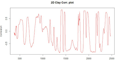
 One of the ways to see which can be the best math treatment for our spectra is to see the correlation plots versus a certain constituent, let´s say "clay" in this case. The "datsoilspc" data set has the reference values for the texture parameters and total carbon, so let´s use clay to calculate the correlation of the second derivative calculated in the previous plot with the clay parameter, and we do its wavelength by wavelength, so we get an spectrum.

The spectra of the second derivative is:

And now we calculate the correlation plot:

cor_spec2d_clay<-cor(datsoilspc$clay,spectra_2d[,1:2098])
matplot(as.numeric(colnames(spectra_2d)),t(cor_spec2d_clay),
type = "l",xlab="nm",col = "red", ylab="Correlation)"
main = "2D Clay Corr. plot")

Due that we are calculating the correlation with the second derivative spectra, we have to look to the negative correlations, and we can see that there are interesting zones (high correlated with clay) after 2000 nm, where clay minerals like "kaolinite" absorb NIR radiation.