R exercises 3.1 (part 2)

As we can see in the previous post, there are highly correlated variables (RI and Ca) and other that we can consider medium or low correlated, and even that are not correlated at all.

In the case of the histograms we can see that some variables are skewed and in some cases it appears that the are some extreme outliers (like in the "K"), but at the moment we does not exclude any of the samples.

We can check with the PCA analysis if there are some transformations which can reduce the number of variables. We can see in the type variable that we have seven classes, so we can check at the same time if we can observe some clusters in the PC space for these classes.

pcaObject<- prcomp(Glass[,1:9], center = TRUE, scale. = TRUE)
#Percent of variance explained for every component
round(pcaObject$sd^2/sum(pcaObject$sd^2)*100, 1)

[1] 27.9 22.8 15.6 12.9 10.2  5.9  4.1  0.7  0.0

As we can see the number of dimensions in the decrease (from 9 to 8) due to the high correlation between two of the variables. Now we can plot the scores maps to see if we can find some clusters.

pairs(pcaObject$x[,1:3], col = Type)

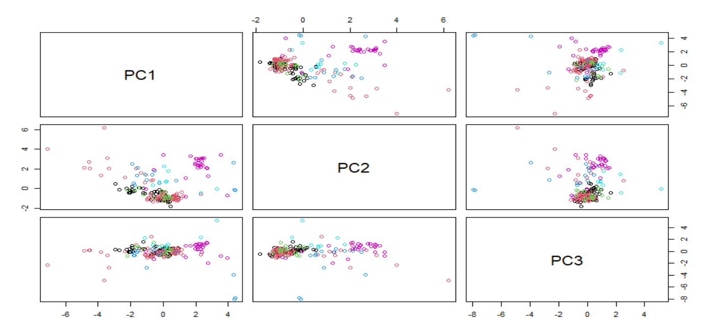
PCA is a not supervised method and we can see possible clusters but with different classes overlapped, so we have to work trying to find some transformations which improve as much as possible the classification methods.

We can use now Caret to reduce improve the skewed  variables and  check if there are some improvement in the classification of types:

library(caret)

trans<- preProcess( Glass[,1:9], 

                    method = c("BoxCox", 

                    "center", "scale", "pca"))

transformed<- predict(trans, Glass)

pairs(transformed[,2:4], col = Type)

We can compare the PC1 vs PC2 score map for both cases

As we can see they are very similar and it does not seem to make so much improvement the PCA and reduction of the skewness to classify correctly some of the groups.