What are the benefits of adding more data to the models?

One of the frequent questions before developing a calibration is: How many samples are necessary to develop a calibration?. The quick answer is: ¡as much as possible!. Of course is obvious that they should content variability and represent as much as possible the new data can appear in the future.

 

The main sources of error are the "Irreducible error" (error from the noise of the instrument itself), the unexplained error (variance) and the Bias and they follow some rules, depending of the number of samples we have. Another thing to take into account is the complexity of the model (the number of coefficients, parameters, or terms we add to the regression).

 

Let´s look to this plot:

Now, if we add more samples tis lines are keep them as dash lines and the Bias, Variance and Total Error improves but the complexity (vertical black line) increase, and this is normal.

 

 

 

Using "tecator" data with Caret (part 3)

This is the third part of the series "Using Tecator data with Caret" , you can read first the posts:

 

Using "tecator" data with Caret (part 1) 

Using "tecator" data with Caret (part 2)

 

When developing the regression for protein, Caret select the best option for the number of terms to use in the regression, so in this case that I have developed two regressions (PCR and PLS), Caret select 11 terms for the PLS regression and 14 for the PCR.

 

This  is normal because in the case of PLS all the terms are selected taking in account how the scores (projections over the terms) correlate with the  reference values for  the parameter of interest, so they rotate to increase as much as possible the correlation value of the scores to the reference values. In the case of PCR the terms explain the variability in the spectra matrix and after a multiple linear regression is developed with these scores and is in this moment when the reference values are take it into account.

 

In this plot I show the XY plot of reference values of predictions vs. reference values for PCR and PLS over-plotted, with a validation set (sample removed randomly for testing the regression)

 

 

The error are similar for both:

 

RMSEP  for PCR..................0,654

RMSEP  for PLS...................0,605

 

 

Using "tecator" data with Caret (part 2)

I continue with the exercise of Tecator data from the :
Chapter 6 | Linear Regression and Its Cousins
in the book Applied Predictive Modelling.

In this exercise we have to develop different types of regression and to decide which performs better.
I use for the exercise math treatments to remove the scatter, in particular the SNV + DT with the package "prospectr".

After I use the "train" function from caret to develop two regressions (one with PCR and the other with PLS) for the protein constituent.

Now the best way to decide is a plot showing the RMSE for the different number of components or terms:

Which one do you thinks performs better?.
How many terms would you choose?

I will compare this types of regressions with others in coming posts for this tecator data.

Using "tecator" data with Caret (part 1)

In the Caret package, we have a data set called “tecator” with data from an Infratec for meat. In the book “Applied Predictive Modelling”, is used as an exercise in the Chapter : “Linear Regression and its Cousins”, so I´m going to use it  in this and some coming posts.

When we develop a PLS equation with the function “plsr” in the “pls” package we get several values, and one of them is “validation”, where we get a list with the predictions for the number of terms selected for the samples in the training set. With these values, several calculations will define the best model, so we does not overfit it.

Anyway, to keep apart a random set for validation will help us to adopt the best decision for the selection of terms. For this, we can use the “createDataPartition” from the Caret package. The “predict” using the developed model and the external validation set will give us the predictions for the external validation set and comparing this values with the reference values we will obtain the  RMSE (using the RMSE) function, so we can decide the number of terms to use for the model we use finally in routine.

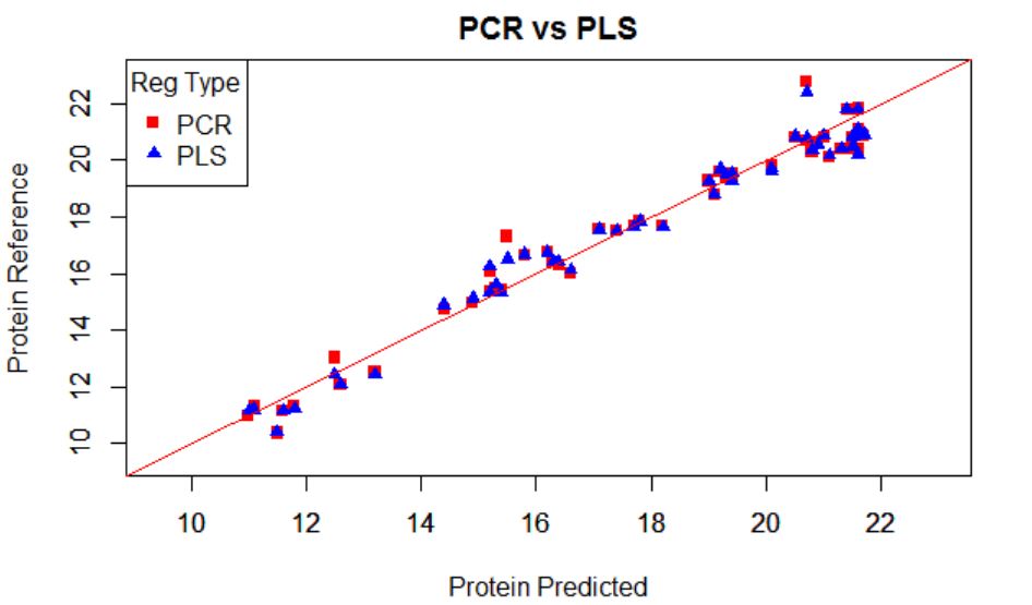
We normally prefer plots to see performance of a model, but the statistics (numbers) will really decide how the performance is.

In the case I use 5 terms (seems to be the best option), the predictions for the training set are:

train.dt.5pred<-plsFitdt.moi$validation$pred[,,5]

In addition, the predictions for the external validation set are:

test.dt.pred<-predict(plsFitdt.moi,ncomp=5,

                      newdata = test.dt$NIR.dt)

With these values we can plot the performance of the model:

plot(test.dt.pred,test.dt$Moisture,col="green",

     xlim=range.moi,ylim=range.moi,

     ylab="Reference",xlab="Predicted")

 

par(new=TRUE)

 

plot(train.dt.5pred,tec.data.dt$Moisture,col="blue",

     xlim=range.moi,ylim=range.moi,

     xlab="",ylab="")

 

abline(0,1,col="red")

Due to the high range of this parameters we can see plots as this, where we can see area ranges with bias, others with more random noise, or others with outliers.

Reconstruction: Residual vs Dextrose

I tried to explain in several posts how the Residual Matrix that remains after apply a Principal Components Algorithm can show us the residual spectra so we can see what else is in an unknown sample analyzed in routine which can not be explained by the Principal Components model.

In this plot I show the residual for three samples which has an ingredient which was not in the model that we build with samples of different batches of a certain formula.

We can correlate the residual spectra with a database of ingredients to have an idea of what could be the ingredient more similar to that residual.

I compare the residual with the spectra of dextrose (in black), and the correlation is 0,6, so it can be a clue that dextrose can be in the unknown sample analyzed.