Soy meal Protein bands

I merged in this case the Excel Plots with the Win ISI spectra to get this picture. We can see in black the raw  and second derivative spectra of a 47% protein soy meal sample. In green the are 2ª derivative spectra of soya hulls and soya beans. All this spectra can help us to understand better this products when developing calibrations.

 Click on the picture to enlarge it.

Removing redundant samples

Sometimes we accumulate huge amounts of spectra in a CAL file, and most of them is redundant and maybe that not helps to improve the calibration. One thing important when we have a lot of spectra is that we have more when we can select and to fill our hypercube in the best way. The option "Select Samples from a Spectra File" in Win ISI help us to select samples which fill the hypercube  with the samples at similar distances between them, so all of them are important in the calculation in the centroid, and there are not groups which makes that the centroid is more closer to them. The number of PCs is also reduced and as we can see comparing these two plots (left: without redundant samples, right: with redundant samples) and maybe we increase the variance explained for the PC terms respect to some constituents in the case we want to develop PC regression. So no discard to use this option to improve the calibrations.

 

Comtrade Webpage

These days I am doing an Online Course of  Python and we are practicing extracting data,  to work with, from a very interesting web page that I want to share with the readers of this blog.
http://comtrade.un.org/data/
From this web page you can extract very interesting information about your country, about from or to where, we import  or exports commodities.
For example in this case I want to see from which countries we imported computers and to which countries we exported computers in 2015:

You can preview or download the csv file and to work with it  R or Python for grouping and practice statistics.
The first row is the result for all the countries in the World. So we have to look to the next rows to see from which countries we import or to which countries we export computers:
In the case of imports:

and in the case of exports:

Hope you find it interesting, and share things that have surprise you from your Country.

Looking to the plots (Validation for W in flour)

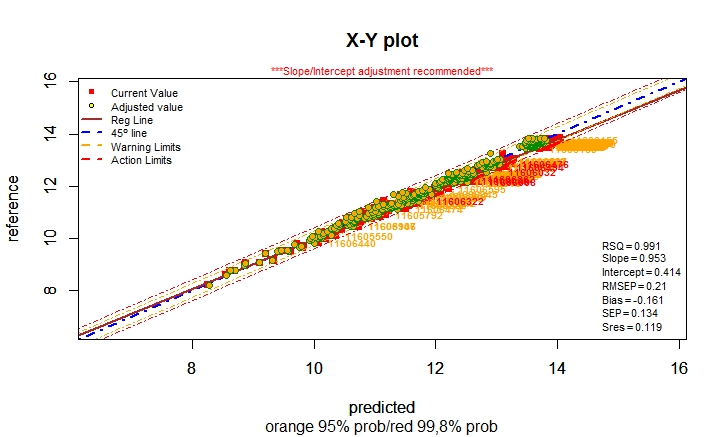
When we check a model with a validation set, what we normally look is to the standard error of prediction (RMSEP) and the RSQ. 

After we check if we have a bias and to the standard error of prediction corrected by bias. Maybe we are happy with the results if we see that are similar to the calibration statistics or maybe not so happy and think that the calibration does not work. 

It is important to check if we have outliers and to remove those samples that could increase the errors, but if they are not clear outliers, they must stay. What we can do is if the error is bigger is some parts of the XY plot.

Maybe the calibration is not so fine for certain range, but it works fine for other range. This way we can take some conclusion about where to include more samples to improve the calibration. 

Histograms will help you with this as well, but also the X-Y plot of reference versus predicted. In the case of flour there are different types according to the W parameter.

In the X-Y plot I can see with an independent validation set that the calibration is performing well for flour between 200 and 270 of W, with a RMSEP of 9. This tells me that the calibration is working fine for this type of flour used normally for pizza products.

The calibration does not work for soft flour (low W) or hard flour (high W). You have to decide how to improve it or to separate the flour product into 3 products in order to improve the predictions.

Look always to the plots and try to find conclusions about the data.

Looking to the external validation statistics (SEV and SEV(C))

Whenever we transfer calibration databases from one instrument to be used in another type of instrument, we use a type of standardization, scanning samples in both instruments and after that we apply the standardization to the data base and make a new calibration. We need to validate this equation with new samples from the new instruments in order to see if the transfer was correct. But it is usual that the equation can underfit or overfit the number of terms used in the PLS Model. So whe we do the validation probably will in some cases some bias effects or a high SEP than expected.

Is it good to develop the equation again using the new spectra with lab values as an external set for validation in order to decide the number of terms we will use in order to prevent the calibration to be under-fitted or over-fitted.

Just look to the statistics values of the SECV and SEV (SEP for the external validation set) and make your decision.

It is important to look at the same time to the SEV and SEV(C) to check that we have not a bias in the prediction of the validation test.

In the statistic list Win ISI recommends 14 terms for a moisture equation, but we can see clearly that is too much, so we can take the decision to take less. What about four?.  Just try.

Looking to the scatter effects with Unscrambler

In the left side of the previous plots, you can see NIT spectra of wheat kernels, that I have download from the database available at:

http://www.models.life.ku.dk/datasets

This web page is very interesting and also the YouTube Chanel where Rasmus Bro (Professor, Dept. of Food Science, University of Copenhagen) explain PCA and PLS concepts with Unscrambler apart from other Chemometric Lessons.

The data is in Matlab and I have to play with it to import it to Unscrambler. Once in Unscrambler I check the option to look to the scatter effects that I saw in an Unscrambler Camo video in YouTube. The video use the new Unscrambler X, but I have the 9.1, and this function to check the scatter effects is also in this old version.

So in the left side we can see the scatter effect for every sample, and it is clear that we have an add effect that we have to remove.

We want to see the chemical effects and not the physical effects like the scatter. So I apply the S. Golay math treatment and look to the effects again and I see this plot:

and something curious happen, because we continue seeing scatter effects in a multiplicative way from the center to the extremes, so SG could help to improve the correlation with the constituent  of interest, but not the scatter removal, so I add to the SG transformation the MSC transformation and we can see how the scatter is almost removed.

Importing WinISI data into Unscrambler

I use the Win ISI "demo.cal" data to export it as an ASCII file, and I tried to import it into the 9.1 Unscrambler version which has the option to import from ASCII, and a window appears to configure how the ASCII file exported from Win ISI is designed.

This way, I have all data in place so I can start to configure the sample and variable sets.

This is a well known sample set so it is quite interesting for a tutorial of Unscrambler.

 

To consider when transfering calibrations or databases (part 2)

When we transfer a calibration or a database from one instrument to other, we know in advance that we have a sample presentation error in the instrument where the calibration comes from, and it is important to know it before you interpret the statistics.

In this case I know the predictions from several samples acquired in two repacks, so the sample result we consider is the average, but in this case we are interested in the individual results of every repack (2 results in this case). So I can calculate the difference of both results for every repack and after that (with all the values) I can calculate the standard deviation to get what I can consider the repacking error.

Notice that I will have a value of standard deviation for every parameter.

So I can compare this value with the errors the monitor function gives to me.

The error packaging for the moisture in wheat for a NIR5000 with natural product cell was 0,11. After an standardization to transfer the database to a DS2500 I get an RMSEP error of 0,21, but I can see that maybe due to the samples chosen for the standardization I have an slope which affects specially to the samples with high moisture. But I can see also that the error once than the slope and intercept are corrected is Sres=0,12 , very similar to the repacking error, so there is a good improvement which makes me challenge to try a better standardization to improve the calibration or database transfer.

To consider when transfering calibrations or databases (part 1)

There are some occasions where we have to transfer equations or databases from one instrument to other and both instruments have a different sample presentation system, so there is no possibility to scan the same sample in the same cuvette. In this case we have to make some repacking form one cuvette to the other at the same time that we scan the sample on the correspondent instrument. 

It is very important that the sample must be as well homogenized as possible between repacks. As you make more repacks there is a higher possibility that the same sample is presented to both instruments so we can make a better standardization.

But which sample must be chosen for the standardization and to make the repacks. One option is to use a sample with an spectra close to the center of the spectral population, in this case we don´t look to their value in moisture , protein and so on. Later when we evaluate the statistics of the transfer we van see that the standardization works fine in a certain range of the moisture range and not so well in other ranges, so we have to consider also the values of the moisture content of the sample we use for the standardization.

In this case we compare the results of two instrument standardized without taking care of the moisture content of the sample/s used for the standardization, and we can see that in the upper range there is a difference and the monitor function recommends a slope adjustment. We can adjust the slope after the standardization but the idea would be to try other standardization using samples in the moisture range and to check a better performance doing this monitor validation again.

Working with the Shootout 2016 data with R (Part 2)

One of the samples in the instrument A2 is a clear outlier and should be removed. Before to proceed we have to apply a math treatment to remove the scatter so we can compare better the spectra of the same samples scanned on the 3 instruments of the same manufacturers, in this case with the instruments A1 , A2 and A3 of the manufacturer A.

 I choose in this case MSC. After applying the MSC I could overplot the spectra of all these instruments, but we won´t see clearly the differences, so the best way to see the spectral differences is to substract the spectra from the samples scanned on one instrument from the spectra of samples scanned in the others, so in this case I can subtract A1 –A2, A1 – A3 and A2 – A3, and to look to the patterns of the spectra.

We can see that when instrument A2 is involved strange difference spectra appears, so this sample will be removed from all the calibration sets from instruments of Manufacturer A.

CalA1A2<-CalSetA1_tC_spec_msc - CalSetA2_tC_spec_msc
    matplot(wavelengths_C,t(CalA1A2),lty=1,type="l",
    + pch=NULL,xlab="nm",ylab="abs",col="red",main="A1-A2")

CalA1A3<-CalSetA1_tC_spec_msc - CalSetA3_tC_spec_msc
    matplot(wavelengths_C,t(CalA1A3),lty=1,type="l",
    + pch=NULL,xlab="nm",ylab="abs",col="red",main="A1 - A3")

CalA2A3<-CalSetA2_tC_spec_msc - CalSetA3_tC_spec_msc
    matplot(wavelengths_C,t(CalA2A3),lty=1,type="l",
     + pch=NULL,xlab="nm",ylab="abs",col="red",main="A2 - A3")