Win ISI 4.8 available for downloading

Win ISI 4.8 is available at www.winisi.com for downloading:

A ZIP file is downloaded with a PDF file (with the instructions for installation, bugs fixed,....),a folder with the prerequisites, and the program files.

Mahalanobis in the PC space (removing redundant) - 2

We have seeing this plot in previous posts, but it is a good occasion to see them again if yo have read the previous post. The function Moutlier from the package chemometrics, have the option to see the outliers,, in the PC space with the normal covariance matrix and the robust covariance matrix. A line is defined for the cutoff value for a certain chi-square distribution, and the samples out are the outliers. Anyway in this example I am considering just two principal components, but when using more PCs, we give just one value for all of them, and it means that maybe a sample is an outlier for one of the PCs, but for the general computation this sample is fine.

A more conservative approach is to put a bigger distance for the cutoff, or a warning an an action cutoff.

In this plot we see the distance respect to the firts two PCs, and we see the same two outliers than in the previous post (four in the case of the Robust Covariance Matrix).

 

But if we consider the PC2 and PC3·, there are not outliers, and all the samples are bellow the cutoff:

This are sample very with certain physical properties, which make them sensitive to be outliers in the first PC, but not in the rest of the PC score maps.

If somebody wants the file to follow the tutorial, just let me know by mail and I will send it to you. The script is on my Github page

 

The chemometric package is the R companion to the book "Introduction to Multivariate Statistical Analysis in Chemometrics" written by K. Varmuza and P. Filzmoser (2009)

 

Mahalanobis in PC space (removing redundat)

In a previous post, we used "prospectr", with the duplex function to select a training set (30 samples), in order to spend less money in lab analysis. This way, we remove redundants spectra, and the selected spectra are well dispersing all around the PC space. Redundant were discarded according to its Neighborhood Mahalanobis distance.

In this plot, we can see the selected samples (red ones), and a Mahalanobis ellipse, considering all the samples with the "drawMahal" function from the package "chemometrics".

If we consider just the red samples (the 30 samples for the training set), the center of the population will be different that with all the samples (156), so we have to calculate the PCs again (their orientation will change), and we can draw a new Mahalanobis  ellipse (97.5 quantile).

As we can see in the plots,  removing the redundantswill give more weigth to the extreme samples, to be retained, and not be consider as outliers.

Selecting samples for lab analysis (part 4)

After the last post, we have a training set with 30 samples to develop a calibration (due to the few samples, this exercise is just a study in order to create a model with more samples in the future), and a test set with another 30 samples. This test set is useful to tune the model as best as we can (math treatments, number of terms,...).

We just try with the parameter protein, developing a PLSR with the Training Set, and after that predicting the Test set. The prediction values for the Test Set are compared with the Test Set Lab values in order to get the performance statistics.

Validation statistics are compared with the Regression statistics.

Finally a model with the Training + Test Set is developed (60 samples).

All the statistics are studied with a monitor function.

See the script and follow the tutorial in Github.

Details of the plots in the monitor function:

Selecting samples for lab analysis (part 3)

I have been using 159 spectra of soya meal in order to select 60 of them to send to the laboratory (imagine that I can only afford to analyze this number due to the high cost of the reference methods). It is obvious that I would like to select a set which represent as better as possible the whole population of these 159 samples. I used the “duplex algorithm" from "prospectr package", which select a “model set” and a “test set”, so I will have 30 on each.

Some days later the result from the “Lab” are here, so I am anxious to check the “summary” and the “histograms”. Normally you have an idea of the range of protein in the soya meal that you received, and this can help you to check if the sample sets are representative. But in this case I have the advantage to have all the lab values for the 159 samples, so let´s see: (green: Histogram of the 159 samples for protein, blue:histogram of the 30 samples for training, violet: histogram of the 30 samples for validation).

             

Some script using "prospectr"

library(prospectr)
hsoja.X<-as.matrix(read.table("clipboard",header=FALSE))
wavelength1<-seq(from=1100.0,to=2499.5, by=0.5)
X.ID<-seq(from=1,to=159, by=1)
colnames(hsoja.X)<-wavelength1
rownames(hsoja.X)<-X.ID
plot(as.numeric(colnames(hsoja.X)),hsoja.X[1,],
   +type="l",xlab="wavelength",ylab="Absorbance")
matplot(wavelength1,t(hsoja.X),type="l")
hsoja.X.bin<-binning(hsoja.X,bin.size=4)
wavelength2<-seq(from=1100,to=2498, by=2)
colnames(hsoja.X.bin)<-wavelength2
matplot(wavelength2,t(hsoja.X.bin),type="l",
ylab="",xlab="Wavelength")
points(as.numeric(colnames(hsoja.X.bin)),
   +hsoja.X.bin[1,],pch=2)
matplot(wavelength1,t(hsoja.X),type="l",ylab="",
   +xlab="Wavelength",col="black")
par(new=T)
hsoja.Xsnv<-standardNormalVariate(X=hsoja.X)
matplot(wavelength1,t(hsoja.Xsnv),type="l",xaxt="n",
   +yaxt="n",ylab="",xlab="",col="blue")
hsoja.Xsnvdt<-detrend(X=hsoja.X,wav=as.numeric(colnames(hsoja.X)))
par(new=T)
matplot(wavelength1,t(hsoja.Xsnvdt),type="l",
xaxt="n",yaxt="n",xlab="",ylab="",col="red")
h.soja.snvdt1d<-t(diff(t(hsoja.Xsnvdt),differences=1,lag=16))
wavelength3<-seq(from=1108,to=2499.5, by=0.5)
par(new=T)
matplot(wavelength3,t(h.soja.snvdt1d),type="l",
   +xaxt="n",yaxt="n",xlab="",ylab="",col="green")
# All the sequence for the plot
matplot(wavelength1,t(hsoja.X),type="l",
   +ylab="",xlab="Wavelength",col="black")
par(new=T)
matplot(wavelength1,t(hsoja.Xsnv),type="l",
   +xaxt="n",yaxt="n",ylab="",xlab="",col=4)
par(new=T)
matplot(wavelength1,t(hsoja.Xsnvdt),type="l",
   +xaxt="n",yaxt="n",xlab="",ylab="",col=2)
par(new=T)
matplot(wavelength3,t(h.soja.snvdt1d),
   +type="l",xaxt="n",yaxt="n",xlab="",ylab="",col="green")
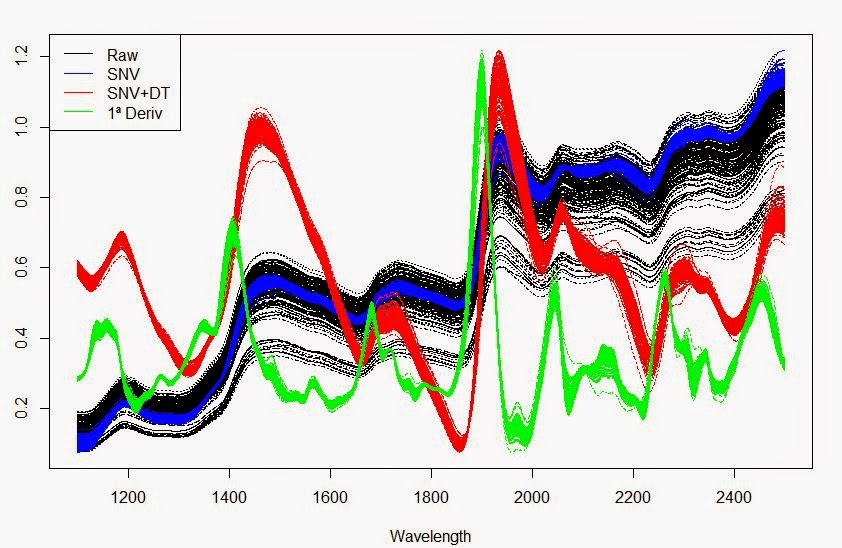
legend("topleft",legend=c("Raw","SNV","SNV+DT","1ª Deriv"),
   +lty=c(1,1),col=c("black","blue","red","green"))