Plotting MIR spectra with ggplot2

 

Loading and preparing the MIR data.

The data is available in the data folder of the repository. Is in a CSV format and can be loaded using the read_csv function from the readr package.

library(readr)

url_mir <- "https://raw.githubusercontent.com/FAO-SID/SoilFER-Spec/main/data/dat2MIR.csv"
dat2MIR <- read_csv(url_mir)

Now we will follow the instructions of the Soil spectroscopy training material changing the name of the first column (index of the samples) to “sample”.

colnames(dat2MIR)[1] <- "sample"
head(dat2MIR, c(10, 7))

# A tibble: 10 × 7
   sample `4001.65608` `3999.72758` `3997.79907` `3995.87056` `3993.94205`
    <dbl>        <dbl>        <dbl>        <dbl>        <dbl>        <dbl>
 1      1       0.180        0.18         0.180        0.180        0.181 
 2      2       0.150        0.151        0.151        0.151        0.151 
 3      3       0.0484       0.0487       0.0489       0.0491       0.0492
 4      4       0.133        0.133        0.133        0.134        0.134 
 5      5       0.227        0.228        0.228        0.228        0.228 
 6      6       0.120        0.120        0.121        0.121        0.121 
 7      7       0.312        0.313        0.313        0.313        0.314 
 8      8       0.225        0.226        0.226        0.226        0.227 
 9      9       0.218        0.219        0.220        0.220        0.221 
10     10       0.113        0.113        0.114        0.114        0.114 
# ℹ 1 more variable: `3992.01354` <dbl>

Looking to the CSV file, we see that the first column is the sample number, and the last one the organic carbon parameter. All the columns in the middle ate the wavenumbers.

Let´s create a vector with the wavenumbers. The wavenumbers are in the column names from the second to the penultimate column, so we can extract them using the following code:

wavenumbers <- as.numeric(colnames(dat2MIR)[2:(ncol(dat2MIR) - 1)])

Let´s prepare the wavenumbers vector to be used as column names in the matrix of spectra.

wavelengths_ir <- round(10000000 / wavenumbers)
wavenumbers_ir <- round(10000000/wavelengths_ir) # Convert to cm-1

my_spectra_ir <- as.matrix(dat2MIR[, 2:(ncol(dat2MIR) - 1)])
colnames(my_spectra_ir) <- wavenumbers_ir

Let´s prepare the MIR dataframe to work with it:

dat_mir <- dat2MIR[, c(1, 1767)]
dat_mir$spc_raw_ir <- my_spectra_ir
rm(my_spectra_ir)

library(tidyverse)

my_wavenumbers <- as.numeric(colnames(dat_mir$spc_raw_ir))

#creating the long dataframe
ir_long <- data.frame(
sample = rep(1:nrow(dat_mir), each = ncol(dat_mir$spc_raw_ir)),
oc = rep(dat_mir$Organic_Carbon, each = ncol(dat_mir$spc_raw_ir)),
wavenumber = rep(my_wavenumbers, nrow(dat_mir)),
absorbance = as.vector(t(dat_mir$spc_raw_ir))
)

head(ir_long)

  sample        oc wavenumber absorbance
1      1 0.7950426       4002    0.17972
2      1 0.7950426       4000    0.18000
3      1 0.7950426       3998    0.18025
4      1 0.7950426       3995    0.18048
5      1 0.7950426       3994    0.18076
6      1 0.7950426       3992    0.18107

We can use the ggplot function to create a plot.

ggplot(ir_long,
       aes(x = wavenumber, y = absorbance, group = sample, color = oc)) +
  geom_line(alpha = 0.5) +
  scale_color_gradient(low = 'blue', high = 'red') +
  scale_x_reverse() +  # Invierte el eje X
  theme_minimal() +
  labs(x = 'Wavenumber (cm⁻¹)',
       y = 'Calculated absorbance',
       color = 'OC (%)')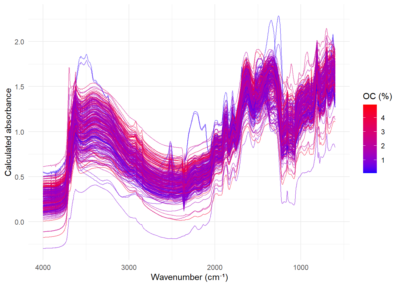

Bibliography:

Soil spectroscopy training material Wadoux, A., Ramirez-Lopez, L., Ge, Y., Barra, I. & Peng, Y. 2025. A course on applied data analytics for soil analysis with infrared spectroscopy – Soil spectroscopy training manual 2. Rome, FAO.

Follow the NIR-Chemometrics blog on Netlify