Ver esta publicación en Instagram

Una publicación compartida por Jose Ramon Cuesta Gonzalez (@jrcuesta)

 

Ver esta publicación en Instagram

Una publicación compartida por Jose Ramon Cuesta Gonzalez (@jrcuesta)

Urban sketching (Museo de Ciencias Naturales)

 

Ejercicio 1: Utilidad de resta de matrices en espectroscopia

Para seguir este espectro se dispone de la matriz de espectros "fish_1_19" que es una matriz de espectros  que preparé en el post anterior y vamos a calcular el espectro medio, simplemente haciendo la media de cada columna (absorbancias a las 19 longitudes de onda) con Excel.

Extendemos la fórmula a las demás longitudes de onda

Y a ese espectro medio lo vamos a llamar el vector "Raw Mean Spectrum" para usarlo a continuación.

Y a continuación hacemos la resta de la matriz "Fish_1_19" de "Raw_Mean_Spectrum".

Simulando espectros de un NIR de 19 filtros en Excel

 A partir de un equipo NIR de rango 400 a 2498 cada dos nanómetros hemos seleccionado las 19 longitudes de onda correspondientes a los 19 filtros de un equipo Bran + Lubbe InfraAlyzer (ver anterior post). Por supuesto que es una gran perdida de datos, pero la idea de los siguientes posts es hacer análisis matriciales más simples para entender conceptos quimiométricos en Excel y de este modo será mucho mas pedagógico.

En este caso usamos un gráfico de scatter por líneas, pero si visualmente lo deseamos podemos quitarlos y poner solo los puntos.

Planificando hacer una base de datos espectral para análisis matricial en Excel.

 En los próximos posts vamos a preparar una matriz de datos espectral con un fichero de demo en el que seleccionaremos 19 longitudes de onda determinadas, simulando ser un equipo NIR de filtros Bran+Luebbe .

Las longitudes de onda serán: 1445, 1680, 1722, 1734, 1759, 1778, 1818, 1940, 1982, 2100, 2139, 2180, 2190, 2208, 2230, 2270, 2310, 2336 y 2348 nm.

1445 (O-H / Agua))

1680-1780  (C-H)             1720 - 1760 (Grasas / Lípidos)

1940 (O-H / Agua)

1980-2180 (N-H / Proteína)

2100 (Almidón / Proteína)

2170 - 2180 (Proteína)

2270-2348 (C-H Combinaciones)

 Con estas selecciones trabajaremos con matrices mas pequeñas y menos intercorrelacionadas para poder entender mejor el análisis quimiométrico en el caso de trabajar con Excel.

Conocimientos básicos: Resta de matrices en Excel

 De gran utilidad es la resta de espectros en quimiometría NIR, por ejemplo, para conocer como ha variado una muestra en el tiempo (restando el espectro actual del original, nos indicará si la muestra a variado en humedad, color,..etc.), o por ejemplo para hacer un centrado espectral que es de lo más común en cálculos de algoritmos como por ejemplo Componentes Principales.

La resta matricial es muy simple en Excel, y usamos a modo de ejemplo las matrices A y B del post anterior:

siendo el resultado:

Conocimientos básicos: Suma de matrices en Excel

 Siguiendo con los temas de matrices en Excel, vamos a realizar en este caso la suma de matrices. Para ello usamos la matriz A del post anterior y vamos a sumarla con otra matriz que debe de cumplir la condición de que tiene el mismo numero de columnas y el mismo número de filas. Si quisiésemos llevar esto al análisis espectral sería como hacer una suma de unos espectros con otros.

Ahora lo que hacemos es definir la nueva matriz como B, seleccionar el rango de columnas y filas adecuado y aplicar la formula A + B, siendo A y B las matrices a sumar:

Al presionar "enter" nos dará el resultado de la suma:

Conocimientos básicos: Definiendo matrices en Excel

 Simplemente rellena un rango de celdas en Excel, si imaginamos que se trata de datos de espectros rellenamos datos un rango k.n, siendo k el numero de puntos de datos y n el número de muestras. En Excel podemos ir a fórmulas y en  el administrados de nombre (Name Manager), lo nombramos con una letra mayúscula, por ejemplo A.

Usemos por ejemplo los datos que aparecen en el libro "Chemometrics in Excel":

Para representarlos gráficamente simplemente seleccionamos la matriz y en Insertar, seleccionamos los gráficos en 2D.

Como veis hemos representado una matriz A y con ella hemos visualizado los espectros. Imaginaros que se trata de un equipo con tres filtros de tres determinadas longitudes de onda y por los que hemos analizado tres muestras. Mas adelante lo haremos con espectros reales de equipos con un mayor numero de longitudes de onda.

Podemos hacer ahora una operación sencilla con esa matriz (multiplicarla por 3). Para ello seleccionamos un rango de celdas de 3.4 y en la primera celda escribimos =3*A y al presionar "enter" nos sale la nueva matriz.

Entender bien como funciona el análisis matricial es importante a la hora de comprender los fundamentos de la quimiometría.

Descarga y trabaja con datos de suelos en NIR

 Una de las páginas donde te puedes descargar datos de espectros de suelos con sus métodos de referencia es en 

ZENODO: Agroscope_SoilSpectralLibrary_2024.

You can download soil spectra analysis to work with from:

ZENODO: Agroscope_SoilSpectralLibrary_2024

Git and Github for R Users

Introduction to machine learning with {tidymodels}

      

How to create the project with all the necessary data to follow the workshop:

1 - In RStudio select: File - New Project - Version Control - Git

2 - In the repository URL paste: https://github.com/nrennie/nhs-r-tidymodels.git

3 - Choose the folder and Create the project

Get started with tidymodels and classification of penguin data

Guía rápida para el uso de tidymodels

Interesante presentación en el grupo de usuarios de R de Madrid para el uso de modelos "tidy" a cargo de Jesús Herranz Valera. 

Podéis descargaros las presentación así como el código que se muestra en la misma desde github.

Iremos comentando el uso de este tipo de modelos en próximos posts.

COMO INTERPRETAR ANÁLISIS DE SUELOS PARTE 1

Digital Soil Spectroscopy

Determinación de fósforo en suelos (Método Olsen)

Standard Normal Variate (SNV)

 As in previous posts, we are going to follow the Soil spectroscopy training material and we are going to use the reference material provided.

Let´s start loading the libraries and the data:

library(tidyverse)
library(prospectr)
load("C:/BLOG/Workspaces/NIR Soil Tutorial/post5.RData")

In the training material we can read a clear explanation of what SNV does:

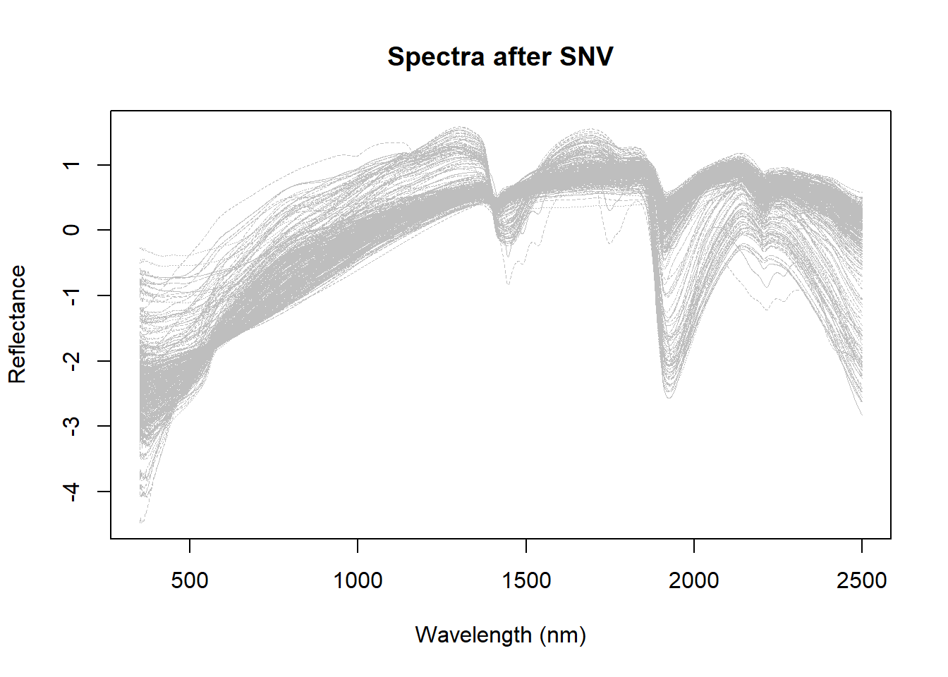
“Standard normal variate is a simple and widely used method that works by centering each individual spectrum to zero and then dividing each spectral band value by the standard deviation of the entire spectrum. The SNV method processes each observation independently. The disadvantage of SNV is that it can be sensitive to noise”.

So for each spectrum we calculate the mean of all data points reflectance values and also their standard deviation. Then we subtract for every data point the mean and divide the result by the standard deviation.

Using the prospectr package, we can use the standardNormalVariate function to apply the SNV transformation to the spectra matrix.

snv_spectra <- standardNormalVariate(dat$spc)

Let´s use first classical R function matplot to plot the spectra before and after the SNV transformation:

matplot(colnames(dat$spc),
  t(snv_spectra),
  type = "l",
  col = "grey",
  lwd = 0.5,
  xlab = "Wavelength (nm)",
  ylab = "Reflectance",
  main = "Spectra after SNV"
)

Now with ggplot2:

# Create the long-format data frame for the different derivatives
snv_spectra_long <- data.frame(
sample = rep(1:nrow(dat), each = ncol(snv_spectra)),
oc = rep(dat$Organic_Carbon, each = ncol(snv_spectra)),
clay = rep(dat$Clay, each = ncol(snv_spectra)),
silt = rep(dat$Silt, each = ncol(snv_spectra)),
sand = rep(dat$Sand, each = ncol(snv_spectra)),
wavelength = rep(my_wavelengths, nrow(snv_spectra)),
absorbance = as.vector(t(snv_spectra))
)


ggplot(snv_spectra_long, aes(x = wavelength, y = absorbance, 
                             group = sample, color = oc)) +
  geom_line(alpha = 0.5) + # Set alpha to 0.5 for transparency
  scale_color_gradient(low = 'blue', high = 'red') +
  theme_minimal() +
  labs(x = 'Wavelength (nm)', y = 'Reflectance', color = 'Organic Carbon (%)')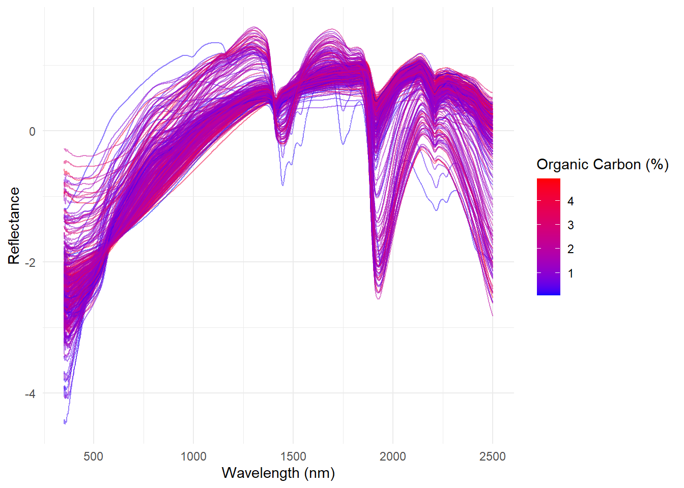

Bibliography:

Soil spectroscopy training material Wadoux, A., Ramirez-Lopez, L., Ge, Y., Barra, I. & Peng, Y. 2025. A course on applied data analytics for soil analysis with infrared spectroscopy – Soil spectroscopy training manual 2. Rome, FAO.

NIR Chemometrics for soil analysis

Adding noise to the spectra

 We have seen in the previous post how to remove artifacts in the spectra using the spliceCorrection function from the prospectr package. But there are other sources of noise in the spectra which depends of several factors, as the quality of the spectrophotometer (can use a signal to noise ratio meassurement to test it), the scanning time, resolution, sample presentation, …. In this post we continue with the “course on applied data analytics for soil analysis with infrared spectroscopy” using the reference material provided. And this time we are going to see the part of the course where we add noise to the spectra and then we apply two methods to remove it. The methods are the Moving Window Average and the Savitzky-Golay Filter.

First we load the libraries we are going to use:

library(tidyverse)
load("C:/BLOG/Workspaces/NIR Soil Tutorial/post4.RData")

Adding noise to the first spectrum

We create some Gaussian noise to the first spectrum in the dataset (mean = 0, standard deviation = 0.0025), and we are gong to add it to the first spectrum in the dataset. Take in account that we are going to select the dataset dat$spc, which is the one we created in the previous post, so we are going to use the spectra without the artifacts.

#Set a seed for reproducibility of random noise
set.seed(801124)
# Add random noise to the first sample’s spectrum
my_noisy_spc <- dat$spc[1, ] + rnorm(ncol(dat$spc), sd = 0.0025)

If we just want to se the noise that we are adding:

ggplot(data = data.frame(wavelength = my_wavelengths, absorbance = rnorm(ncol(dat$spc), sd = 0.0025)),
       aes(x = wavelength, y = absorbance)) +
  geom_line(color = "blue") +
  labs(title = "Noisy Spectrum",
       x = "Wavelength (nm)",
       y = "Absorbance") +
  theme_minimal()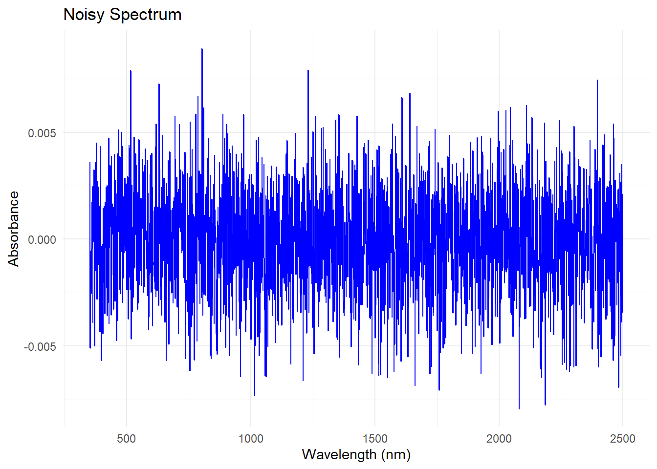

Plotting the noisy spectrum

ggplot(data = data.frame(wavelength = my_wavelengths, absorbance = my_noisy_spc),
       aes(x = wavelength, y = absorbance)) +
  geom_line(color = "blue") +
  labs(title = "Spectrum 1 with added Noise",
       x = "Wavelength (nm)",
       y = "Absorbance") +
  theme_minimal()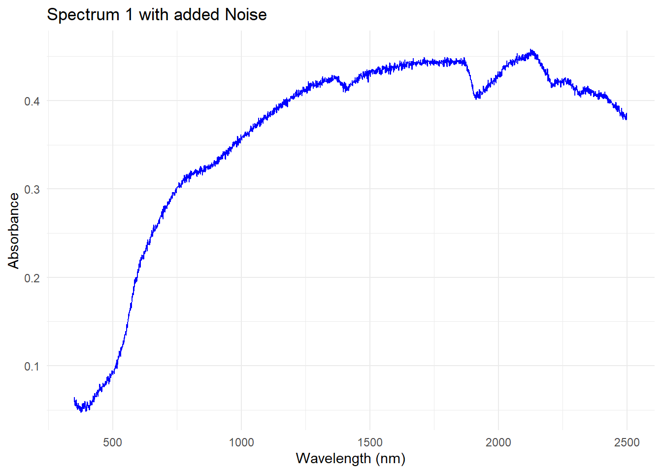

Removing the noise

No let´s apply to this spectrum two methods used to remove noise:

Moving Window Average

library(prospectr)
# Replace ‘my_noisy_spc’ with your actual data frame or matrix and ‘w’ with the desired
# window size
mwa_result <- movav(my_noisy_spc, w = 11)

Savitzky-Golay Filter

# Replace ‘my_noisy_spc’ with your actual data frame or matrix, ‘m’ with the window size,
# and ‘p’ with the polynomial order
sg_result <- savitzkyGolay(
my_noisy_spc, # the noisy spectrum
m = 0, # this m is for the derivative order, 0 is for no derivative
p = 3, # the polynomial order
w = 11 # the window size
)

# Create a long-format data frame for the MVA spectrum
long_mwa_spc <- data.frame(
wavelength = as.numeric(names(mwa_result)), # Extract the wavelengths
spectral_value = mwa_result, # Store the spectral values from the MVA
method = 'mva' # Label the data
)
# Create a long-format data frame for the Savitzky-Golay (SG) spectrum
long_sg_spc <- data.frame(
wavelength = as.numeric(names(sg_result)), # Extract the wavelengths
spectral_value = sg_result, # Store the spectral values from the SG
method = 'sg' # Label the data
)
# Combine the long-format MVA and SG data frames into one
denoised_long <- rbind(long_mwa_spc, long_sg_spc)

Now we create a data frame for the original noisy spectrum and some labels.

# Create a data frame for the original noisy spectrum
original_noisy <- data.frame(
wavelength = my_wavelengths, # Use the original wavelengths
spectral_value = my_noisy_spc # Use the original noisy spectrum values
)

my_labels <- c(
'mva' = 'Moving average smoothing',
'sg' = 'Savitzky-Golay filtering'
)

Now we want to overplot the corrected spectra over the noisy one:

# Plot the spectra using ggplot2
ggplot() +
# Plot the original noisy spectrum as a red line in the background
geom_line(
data = original_noisy,
aes(x = wavelength, y = spectral_value),
color = 'black'
) +
# Plot the MVA and SG processed spectra on top of the original noisy spectrum
geom_line(
data = denoised_long,
aes(x = wavelength, y = spectral_value, color = method, group = method)
) +
# Add titles and labels for the axes
labs(
x = 'Wavelength (nm)',
y = 'Reflectance'
) +
#coord_cartesian(xlim = c(1500, 1800), ylim = c(0.425, 0.450)) +
# Manually set the colors for the MVA and SG lines
scale_color_manual(
values = c('mva' = '#00AFBB', 'sg' = '#E7B800'),
labels = my_labels
) +
# Facet the plot by the method, creating separate plots for MVA and SG
facet_grid(. ~ method, labeller = labeller(method = my_labels)) +
theme(legend.position = 'top') + guides(color = guide_legend(title = NULL))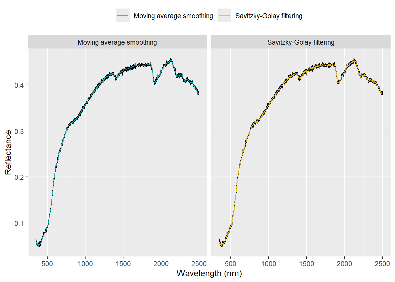

We can zoom the spectra to see the differences more clearly:

ggplot() +
# Plot the original noisy spectrum as a red line in the background
geom_line(
data = original_noisy,
aes(x = wavelength, y = spectral_value),
color = 'black'
) +
# Plot the MVA and SG processed spectra on top of the original noisy spectrum
geom_line(
data = denoised_long,
aes(x = wavelength, y = spectral_value, color = method, group = method), size = 1
) +
# Add titles and labels for the axes
labs(
x = 'Wavelength (nm)',
y = 'Reflectance'
) +
coord_cartesian(xlim = c(1500, 1800), ylim = c(0.425, 0.450)) +
# Manually set the colors for the MVA and SG lines
scale_color_manual(
values = c('mva' = '#00AFBB', 'sg' = '#E7B800'),
labels = my_labels
) +
# Facet the plot by the method, creating separate plots for MVA and SG
facet_grid(. ~ method, labeller = labeller(method = my_labels)) +
theme(legend.position = 'top') + guides(color = guide_legend(title = NULL))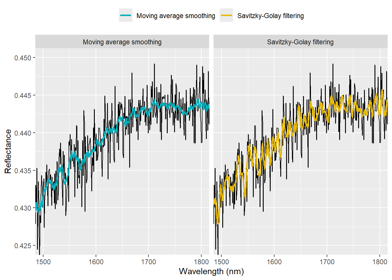

Bibliography:

Soil spectroscopy training material Wadoux, A., Ramirez-Lopez, L., Ge, Y., Barra, I. & Peng, Y. 2025. A course on applied data analytics for soil analysis with infrared spectroscopy – Soil spectroscopy training manual 2. Rome, FAO.