Comparing Residuals an Lab Error

One important point before  develop a calibration is to know the laboratory error. This error, known as SEL (Standard Error Laboratory).

This error change depending of the product, because it can be very homogenous or heterogeneous, so in the first case the lab error is lower than in the second case.

In the case of meat meal the error are higher than for other products and this is a case where I am working these days and I want to share in this posts.

A certain number of samples (n) well homogenized had been divided into two or four subsamples and had been send to a laboratory for the Dumas Protein analysis. After receive the results, a formula used for this case, based on the standard deviation of the subsamples and in the number of samples, gives the laboratory error for protein in meat meal.

The result is 1,3 . Probably some of you can think that this is a high value, but really, the meat meal product is quite complex and I think is normal.

 

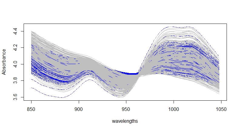
Every subsample that went to the lab has been analyze in a NIR, and the spectra of the subsamples studied apart with the statistic RMS that shows that the samples were well homogenized.

Now I have the option to average the predictions of the NIR predictions (case 1), or to average the spectra of the subsamples, predict it with the model and get the predicted result (case 2). I use in this case the option 1 and plot a residual plot with the residuals of the average predictions subtracted from the lab average value:

Blue line is +/- “ 1.SEL”, yellow +/- “ 2.SEL” and red +/- “ 3.SEL”.

 



 

Monitoring LOCAL calibrations (part 2)

Following with the previous post when monitoring LOCAL equations we have to consider several points. Some of them could be.

1. Which is the reference method and what is the laboratory error for the reference method. Ex:Reference method for protein can be from Dumas or from Kjeldahl .
2. Do you have data from several laboratories or from just one?. Which reference method use every lab and what is their laboratory error. 
3. If we have data in the Monitor from both methods, or from different laboratories, split them apart and see which error  SEP do we have. Check also the SEP corrected by the Bias.
4. Check the performance of the SEP and other statistics for every specie. In meat meal for example you have pork, mix, poultry, feather,....

Sure you can find more knowledge about the data:

1. Do we have more error with one method than another, with one lab than another?.
2. Does perform a reference method better for one particular specie than another?.
3. ................................

Make conclusions from these and other thoughts.

 

For all these, is important to organize well the data and use it fine. Don´t forget that we are comparing reference versus predicted, and that the prediction depends of the model itself apart from the reference values, so we have to be sure that our model is not overfitted or wrong developed.

Monitoring LOCAL calibrations

Databases to develop Local calibrations has normally a high quantity of spectra with lab values, but we have to take care of  them adding new sources of variance. This way we make them more robust and the standard prediction errors (SEP) decrease when we validate with future independent validation sets.

 

This was the case with a meat meal local database updated with 100 samples with protein values, and with new source of variation as: laboratories,  reference methods (Kj, Dumas), providers, new instruments,...

 

After the LOCAL database update, a set of new samples was received with reference values and I have predicted this values with the Monitor function in Win ISI with the LOCAL database before (blue dots) and after the LOCAL update (red dots).

 

The errors decrease , specially for some types of samples, in an important way when validating with the new set of samples (new samples acquired after the updated Local calibration was installed in the routine software), so even if we have spectra from this instrument, labs, ...., this set has to be considered as an independent set.

 

I don´t give details of the statistics but this picture show the same samples predicted with the LOCAL calibration without update (in blue), and predicted with the LOCAL calibration update (in red), the improvement for the prediction for some samples is important, so the idea is to add this new samples and continuing monitoring the LOCAL database with future validation sets.

Nils Foss died on 16-May-2018

Sad news from FOSS: Nils Foss (Foss founder) died yesterday.
He was an good example of entrepreneur.
R.I.P.

Random selection before calibration.

Following a course about Machine Learning with R, I realize of the importance of the random selection of the samples for the development of the models.

R has good tools to select the samples randomly and to do it was a common practice during all the exercises in the course.

 

I do it, in the case with the soy meal samples I have used for several posts, so we will compare the results.

 

The idea of random selection is to make the model robust against the bias which we see quite often when validating the models with independent samples.

 

We can see if the number of the terms selected change or if we get similar results to the previous selection using an structure selection of odd and even samples.

 

Random selection order is important also for a better cross validation.

 

Here is the code and preparation of the sample sets for the development of the models.

##################### SPLITTING SAMPLES RANDOMLY #############  
#In this case we need first the dataframe "soy_ift_conv"
#Split the data into 65% training and 35% test
rndIndices=sample(nrow(soy_ift_conv))
sepPnt=round(.65*nrow(soy_ift_conv))
train=soy_ift_conv[rndIndices[1:sepPnt],]
validation=soy_ift_conv[rndIndices[(sepPnt+1):length(rndIndices)],]
#Plotting Training and Validation sets overlapped.
matplot(wavelengths,t(train$X_msc),type="l",
              xlab="wavelengths",ylab="Absorbance"
              ,col="blue")
par(new=TRUE)
matplot(wavelengths,t(validation$X_msc),lty=1,
        pch=NULL,axes=FALSE,
        type="l",col="gray",xlab="",ylab="")

We see in gray the validation samples selected and in blue the training samples.

        

First approach to ANN calibrations

This is a first approach to develop ANN calibrations with the soymeal data from Infratec and it is really promising.
I follow this code and plot the results:

#We build a dataframe with the constituent values
#and with the spectra math treated with MSC
Sample<-sm_ift[,1]
Y<-as.matrix(sm_ift[,2])        # La matriz Y son los datos de proteina.
which(is.na(Y), arr.ind=TRUE)   # La 462 tiene por valor NA y la quitamos
Y<-Y[-462,]
X<-as.matrix(sm_ift[,6:105]) # La matriz X son los datos NIR
X<-X[-462,]
library(ChemometricsWithR)
library(pls)
X<-msc(X)
##====================================================================
##PRINCIPAL COMPONENTS ANALYSIS using package "Chemometrics" NIPALS)
##====================================================================
library(chemometrics)
X_nipals<-nipals(X,a=4)
T<-X_nipals$T
T<-round(T,4)
T1<-T[,1]
T2<-T[,2]
T3<-T[,3]
T4<-T[,4]
P<-X_nipals$P
P<-round(P,4)
###################################################################
soymeal=data.frame(T1=T1,T2=T2,T3=T3,T4=T4,Y=Y)
#' Split the data into 65% training and 35% test
rndIndices=sample(nrow(soymeal))
sepPnt=round(.65*nrow(soymeal))
train=soymeal[rndIndices[1:sepPnt],]
test=soymeal[rndIndices[(sepPnt+1):length(rndIndices)],]
#' Create an neural network model with 3 hidden
#' nodes of Y~. using the training data.
#' Store this model as 'model'
library(datasets)
library(nnet)
library(graphics)
model=nnet(Y~.,train,size=4,linout=T)
#' Use this model to estimate the Y values of the test data
pre=(predict(model,test))
pre=round(pre,2)
#' Calculate the MSE of the model on the test data and output
#' it using the print or cat functions
mse=mean((test$Y-pre)^2)
cat("The MSE of the model on the test data is: ",mse,"\n")
#The MSE of the model on the test data is:  0.9314747
plot(pre,test$Y)
abline(0,1)

The loss function in this case is MSE (Mean Square Error).
More practice these coming days