Foss Calibrator (quick mPLS overview)

I am starting to use the new software Foss Calibrator, so I will publish some posts about how it works. I use in this case the software for some samples of meat for a viability study of the calibration, and the software improves the split of the sample set into a validation and a calibration set, giving several options like random, time based,...We can choose also if the validation set is into the range of the calibration set, so the model has all the validation samples into the range of the constituent calibration, this way we have quickly the calibration and validation set ready to develop the calibration.

 

For the calibration we have several options for the cross validation (leave one out, using blocks, venetian blinds,......).

We can choose for developing the calibration the options: mPLS, PLS, ANN or LOCAL.I try for this case the mPLS models.

We can select the wavelength range, so we have to look to the spectra to see how if looks and remove noisy part of the spectra, or remove the visible part,.....

The XY plot of Measured vs Predicted shows the calibration and validation samples overlapped and is quite useful for a quick idea of the performance of the model.

 

We have also the plot of the GH distances with the calibration and validation values overlapped:

 

We see the statistics of the model and this time the RMSEP is the total error and the SEP is the error with the bias correction which makes easier to compare the results with other software or literature.

 

 

We can publish the model (calibration and outlier model together) to a folder in our PC and get the ".eqa", ".pca", and ".lib" files to use in Win ISI or load in MOSAIC Network or Solo, and get a report of the calibration.

 

I will continue sharing my experience with Foss Calibrator with the Label "Learning Foss Calibrator"

"R" en la Jornadas Técnicas NIR de FOSS

El pasado martes 27 de Noviembre se celebraron en Madrid la Jornadas Técnicas NIR de FOSS, un evento anual en el que FOSS presenta en España las nuevas tendencias de la instrumentación NIR en FOSS que van dirigidas a la digitalización con productos como el "Foss Assure", "Mosaic" y "Foss Calibrator" entre otros. Con ellos el DS2500 o DA1650 (entre otros) se están convirtiendo en productos que van a poder beneficiarse de estas herramientas digitales e ir evolucionando con ellas.

Foss Calibrator será la nueva plataforma de calibración que sucederá a Win ISI en un futuro próximo. Por supuesto Win ISI ha estado presente en las Jornadas y también ha sido para mí un placer que "R" lo estuviese en mi ponencia.

"R" despertó un gran interés de lo cual me alegro, ya que los usuarios de este software deseamos promocionarlo para que se vea y use el enorme potencial que tiene.

Un placer escuchar a @jrcuesta hablando de NIR y Quimiometria en la Jornada Técnica NIR de FOSS. Siempre se aprende algo nuevo. pic.twitter.com/GMHUNQbdjr

— SECRAN (@SECRAN3) 27 de noviembre de 2018

Variable Importance in NIR "PLS" Models (CARET)

This is a function of the R Caret package to check the importance of the variables in a regression. In the case of the model developed with the sunflower seed to determine oleic acid (model_oleic), we can plot it and check which variables have more importance and this is done with a simple step:

 

varImp_pls<-varImp(model_oleic)

 

And the best way to check it is plotting the results as a spectrum:

 

matplot(wavelengths,varImp_pls$importance,type="l",
        xlab="wavelengths",
        ylab="importance",
        ylim =c(min(varImp_pls$importance)-0.1,
                max(varImp_pls$importance)+0.1),
        col="blue")

 

To obtain this spectra:

We can see that the zone of 1700 to 1800 has higher important than the rest due to the peaks linked to the "oil" around 1720 and 1760 nm.

 

¿Cuando los resultados que predice el NIR son fiables?

Esta es una de las preguntas más comunes que se hacen los usuarios del NIR y que voy a tratar de simplificar una respuesta.

Cuando se instala un modelo de calibración, este lleva unos estadísticos que indican los errores de la calibración, y se conocen como:

SEC (Error Estándar de Calibración) y SECV (Error Estándar de Validación Cruzada)

 

Posteriormente a la instalación de la ecuación para su uso en rutina, y cuando ya tenemos unas 20 muestras de cada parámetro, podemos calcular el SEP (Error Estándar de Predicción) y hacer una comparativa de los tres errores para sacar conclusiones. La situación ideal es cuando los tres estadísticos de error son parecidos y lo suficientemente bajos como para poder usar la aplicación por NIR .

 

Tenemos que tener en cuenta que conocer el error de laboratorio (SEL) nos ayudará a conocer el ratio de error entre el NIR y el Laboratorio y tomar también decisiones para ver como bajarlo (presentando la muestra de modo diferente,....,etc).

Cuando validamos y calculamos el SEP, podemos generar otros estadísticos para ver si la ecuación se está comportando correctamente o no, basándonos en la ecuación que tenemos instalada y para ello se necesitan el número de muestras que hay en la calibración instalada así como el número de términos que se usó, el nivel de confianza que queremos y el SEC o SECV. Con ello se generan unos limites de confianza para el Bias, la Pendiente y el SEP. En el caso de que los resultados estén dentro de los límites, podemos seguir usando el modelo con confianza en los márgenes de error dados inicialmente.

 

Este es un ejemplo:

En un modelo para Oleico en pipa de Girasol molida (con molino de tipo Moulinex), con 109 muestras, 5 términos , un nivel de confianza de 95% y un SECV de 2,21 los resultados del test de la ISO 12099:2010 son:

 

 

Como podemos comprobar el SEP está dentro de los límites previstos y el modelo puede seguir siendo usado. No obstante tenemos que sacar conclusiones para ver como mejorarlo, y el XY plot nos puede ayudar:

 

Parece probable que con una mejora en la molienda de la muestra, con replicados, u otros métodos de presentación el modelo puede ser mejorado, pero tal como se está realizando actualmente es operativo.

Confusion Matrix with Caret

This is a useful tool in R in order to evaluate a predictive model for classification. We know the expected value and the predicted on and from that we can get the Confusion Matrix and the useful statistics based by formulas from that matrix.
I reproduce here the code from the post: "How To Estimate Model Accuracy in R Using The Caret Package"  from the blog "Machine Learning Mastery":

# load the libraries
library(caret)
library(klaR)
# load the iris dataset
data(iris)
# define an 80%/20% train/test split of the dataset
split=0.80
trainIndex <- createDataPartition(iris$Species,
                                  p=split,
                                  list=FALSE)
data_train <- iris[ trainIndex,]
data_test <- iris[-trainIndex,]
# train a naive bayes model
model <- NaiveBayes(Species~., data=data_train)
# make predictions
x_test <- data_test[,1:4]
y_test <- data_test[,5]
predictions <- predict(model, x_test)
# summarize results
confusionMatrix(predictions$class, y_test)

Try to understand the results, some samples are well classified and others not. So we must try to find the model where we have the better statistics for the classification. This is a simple example, but why not to try this machine learning algorithms to spectra for classification and use the confusion matrix to get the best model.
The statistics we get running the last line of code are:

> confusionMatrix(predictions$class, y_test)
Confusion Matrix and Statistics

            Reference
Prediction   setosa versicolor virginica
  setosa         10          0         0
  versicolor      0          9         1
  virginica       0          1         9

Overall Statistics
                                          
               Accuracy : 0.9333          
                 95% CI : (0.7793, 0.9918)
    No Information Rate : 0.3333          
    P-Value [Acc > NIR] : 8.747e-12       
                                          
                  Kappa : 0.9             
 Mcnemar's Test P-Value : NA              

Statistics by Class:

                     Class: setosa Class: versicolor Class: virginica
Sensitivity                 1.0000            0.9000           0.9000
Specificity                 1.0000            0.9500           0.9500
Pos Pred Value              1.0000            0.9000           0.9000
Neg Pred Value              1.0000            0.9500           0.9500
Prevalence                  0.3333            0.3333           0.3333
Detection Rate              0.3333            0.3000           0.3000
Detection Prevalence        0.3333            0.3333           0.3333
Balanced Accuracy           1.0000            0.9250           0.9250

An easy example to understand the confusion matrix can be with this code:
library(caret)
expected <- factor(c(1, 1, 0, 1, 0, 0, 1, 0, 0, 0))
predicted <- factor(c(1, 0, 0, 1, 0, 0, 1, 1, 1, 0))
results <- confusionMatrix(data=predicted, reference=expected)
print(results)
Where you get:

> print(results)
Confusion Matrix and Statistics

          Reference
Prediction 0 1
         0 4 1
         1 2 3
                                          
               Accuracy : 0.7             
                 95% CI : (0.3475, 0.9333)
    No Information Rate : 0.6             
    P-Value [Acc > NIR] : 0.3823          
                                          
                  Kappa : 0.4             
 Mcnemar's Test P-Value : 1.0000          
                                          
            Sensitivity : 0.6667          
            Specificity : 0.7500          
         Pos Pred Value : 0.8000          
         Neg Pred Value : 0.6000          
             Prevalence : 0.6000          
         Detection Rate : 0.4000          
   Detection Prevalence : 0.5000          
      Balanced Accuracy : 0.7083   

From the Caret Documentation which are the formulas for these statistics:

Building Predictive Models in R Using the caret Package

I recommend the reading and practice of the paper :

Building Predictive Models in R Using the caret Package

you can follow the Tutorial with the Mutagen Data in R is a good practice.
The code is in the paper, but in some cases we have to work with R to do certain steps like the code in red.

library(caret)
set.seed(1)
in.Train<-createDataPartition(mutagen,p=3/4,list=FALSE)
trainDescr<-descr[in.Train,]              #used for model training
testDescr<-descr[-in.Train,]               #used to evaluate model performance
trainClass<-mutagen[in.Train]           #used for model training
testClass<-mutagen[-in.Train]           #used to evaluate model performance
prop.table(table(mutagen))                #distribution mutagen all
prop.table(table(trainClass))             #distibution of the training set
#There were three zero{variance predictors in the training data.
sum(apply(trainDescr, 2, var) == 0)     # 3
variance<-apply(trainDescr, 2, var)
zv<-variance==0
which(zv, arr.ind = TRUE, useNames = TRUE)
#T.F..Br. G.F..Br.    I.097
#155      708         1539
trainDescr<-trainDescr[,-c(155,708,1539 )]  #zero variance descriptors removed
testDescr<-testDescr[,-c(155,708,1539 )]    #zero variance descriptors removed
#We also remove predictors to make sure that there are no
#between-predictor (absolute) correlations greater than 90%:
ncol(trainDescr)                        #1576
descrCorr<-cor(trainDescr)              #Correlation Matrix   1579.1579
highCorr<-findCorrelation(descrCorr,0.90)
#Remove the high correlated descriptors from the Training and Test sets
trainDescr<-trainDescr[,-highCorr]
testDescr<-testDescr[,-highCorr]
ncol(trainDescr)                        #650

CARET:Splitting Based on the Predictors

I´m practicing with CARET, and the best way is to follow the tutorials in the webpage. This time is the way how we can split the data with Caret:

4.2:Splitting Based on the Predictors

Read and try to understand the concept.
I try to write the code of the plot for the plot  of the figure, and finally more or less I do it:

testing <- scale(BostonHousing[, c("age", "nox")])
set.seed(5)
## A random sample of 5 data points
startSet <- sample(1:dim(testing)[1], 5)
samplePool <- testing[-startSet,]
start <- testing[startSet,]
newSamp <- maxDissim(start, samplePool, n = 20)
newSamp<-samplePool[newSamp,]
rownames(newSamp)<-c(1:20)
plot(samplePool[,1],samplePool[,2],pch=20,
     col="grey",xlim=c(-2.500,1.400),
     ylim=c(-1.600,2.900),xlab="age",ylab="nox")
par(new=TRUE)
plot(start[,1],start[,2],pch="S",
     col="red",xlim=c(-2.500,1.400),
     ylim=c(-1.600,2.900),xlab="",ylab="",cex=1.3, font=2)
par(new=TRUE)
plot(newSamp[,1],newSamp[,2],col="blue",xlim=c(-2.500,1.400),
     ylim=c(-1.600,2.900),xlab="",ylab="")
text(newSamp[,1],newSamp[,2],
     labels=rownames(newSamp),cex=1.3,     
     font=2)

The samples chosen are different because of the random order. See how the distribution of the chosen samples cover the structure of the data.

PCA with Caret

In this plot we test different types of Principal Components Analysis with different packages. This time I use Caret.

I use the same Tecator Meat data which comes with the package. Spectra is treated with MSC  (Multiple Scatter Correction) and I represent the plane of the scores with the two terms chosen by the PCA processing:

absorp_pca<-preProcess(absorpTrainMSC,
                       method = c("center", "scale","pca"),
                       thresh = 0.95)
PC_scores_train<-predict.preProcess(absorp_pca,absorpTrainMSC)
plot(PC_scores_train[,1],PC_scores_train[,2],col="blue",
     xlim=c(-15,11),ylim = c(-20,11),
     xlab = "PC1",ylab = "PC2")
PC_scores_test<-predict.preProcess(absorp_pca,absorpTestMSC)
par(new=TRUE)
plot(PC_scores_test[,1],PC_scores_test[,2],col="red",
     xlim=c(-15,11),ylim = c(-20,11),
     xlab = "",ylab="")

Now we get the plot of the scores for the training set in blue and for the test set in red.

Playing with CARET and TECATOR MEAT DATA

###### LOADING TECATOR DATA ###################################
library(caret)
library(pls)
data(tecator)
#' Loading the tecator data we load two matrices:
    #' The spectra matrix "absorp" (raw spectra)
    #' We want to create another matrix with MSC math treatment
    absorpMSC<-msc(absorp)
    #' The constituents matrix "endpoints (Moisture, Fat & Protein)
set.seed(930)
#We can add names to the columns with the wavelengths values.
wavelengths<-as.matrix(seq(850,1048,by=2))
colnames(absorp)<-wavelengths
colnames(endpoints)<- c("Moisture","Fat","Protein")
#' We will model the protein content data and create a data partition
#' leaving 3/4 for the training set and 1/ for the validation set.
#' With the createDataPartition we generate a selection of sample positions
#' in a ramdon order to take after this samples out from the absorp and
#' endpoint matrices. 
###### SPLITTING THE DATA #####################################
trainMeats <- createDataPartition(endpoints[,3], p = 3/4)
#'Now we select the correspondant training and validation matrices
#'with the raw and MSC treated spectra
absorpTrain  <- absorp[trainMeats[[1]], ]
absorpTrainMSC<-as.matrix(absorpMSC[trainMeats[[1]], ])
absorpTest   <- absorp[-trainMeats[[1]], ]
absorpTestMSC   <- as.matrix(absorpMSC[-trainMeats[[1]], ])
#########  RAW SCAN SPECTRA  ##################################################
matplot(wavelengths,t(absorpTrain),type="l",
        xlab="wavelengths",ylab="Absorbance",col="blue")
par(new=TRUE)
matplot(wavelengths,t(absorpTest),type="l",
        xlab="",ylab="",col="green")
#########  MSC SCAN SPECTRA  ##################################################
matplot(wavelengths,t(absorpTrainMSC),type="l",xlab="wavelengths",
        ylab="transmitance",ylim =c(min(absorpTrainMSC)-0.1,
                                    max(absorpTrainMSC)+0.1),
        col="blue")
par(new=TRUE)
matplot(wavelengths,t(absorpTestMSC),type="l",xlab="wavelengths",
        ylab="transmitance",ylim =c(min(absorpTrainMSC)-0.1,
                                    max(absorpTrainMSC)+0.1),
                                    col="green")
#'and from the endpoint matrix for every constituent
moistureTrain <- endpoints[trainMeats[[1]], 1]
fatTrain <- endpoints[trainMeats[[1]], 2]
proteinTrain <- endpoints[trainMeats[[1]], 3]
# The rest of the samples go to the Validation Set
moistureTest <- endpoints[-trainMeats[[1]],1]
fatTest <- endpoints[-trainMeats[[1]], 2]
proteinTest  <- endpoints[-trainMeats[[1]], 3]
#We can combine these two matrices:
  # For Protein
trainDataProt<-cbind(proteinTrain,absorpTrain)         #Protein Raw Training
testDataProt<-cbind(proteinTest,absorpTest)            #Protein Raw Test
trainDataProtMSC<-cbind(proteinTrain,absorpTrainMSC)   #Protein Raw Training
testDataProtMSC<-cbind(proteinTest,absorpTestMSC)      #Protein Raw Test  
  #For Fat
trainDataFat<-cbind(fatTrain,absorpTrain)               #Fat Raw Training
testDataFat<-cbind(fatTest,absorpTest)                  #Fat Raw Test
trainDataFatMSC<-cbind(fatTrain,absorpTrainMSC)         #Fat MSC Training
testDataFatMSC<-cbind(fatTest,absorpTestMSC)            #Fat MSC Test
  #For Moisture
trainDataMoi<-cbind(moistureTrain,absorpTrain)          #Moisture Raw Training
testDataMoi<-cbind(moistureTest,absorpTest)             #Moisture Raw Test
trainDataMoiMSC<-cbind(moistureTrain,absorpTrainMSC)    #Moisture MSC Training
testDataMoiMSC<-cbind(moistureTest,absorpTestMSC)       #Moisture MSC Test
#####  BUILDING THE MODELS ####################################
#####  MODELS FOR MOISTURE
model_moi_raw <- train(moistureTrain~.,data=trainDataMoi, method = "pls",
               scale = TRUE,
               trControl = trainControl("cv", number = 10),
               tuneLength = 20)
model_moi_msc <- train(moistureTrain~.,data=trainDataMoiMSC, method = "pls",
               scale = TRUE,
               trControl = trainControl("cv", number = 10),
               tuneLength = 20)
#####  MODELS FOR FAT
model_fat_raw <- train(fatTrain~.,data=trainDataFat, method = "pls",
                       scale = TRUE,
                       trControl = trainControl("cv", number = 10),
                       tuneLength = 20)
model_fat_msc <- train(fatTrain~.,data=trainDataFatMSC, method = "pls",
                       scale = TRUE,
                       trControl = trainControl("cv", number = 10),
                       tuneLength = 20)
#####  MODELS FOR PROTEIN
model_prot_raw <- train(proteinTrain~.,data=trainDataProt, method = "pls",
                   scale = TRUE,
                   trControl = trainControl("cv", number = 10),
                   tuneLength = 20)
model_prot_msc <- train(proteinTrain~.,data=trainDataProtMSC, method = "pls",
                   scale = TRUE,
                   trControl = trainControl("cv", number = 10),
                   tuneLength = 20)
######  PREDICTIONS ########################################
## PROTEIN PREDICTIONS
pred_prot_test_raw <- predict(model_prot_raw,testDataProt)
pred_prot_test_msc <- predict(model_prot_msc,testDataProtMSC)
## FAT PREDICTIONS
pred_fat_test_raw <- predict(model_fat_raw,testDataFat)
pred_fat_test_msc <- predict(model_fat_msc,testDataFatMSC)
## MOISTURE PREDICTIONS
pred_moi_test_raw <- predict(model_moi_raw,testDataMoi)
pred_moi_test_msc <- predict(model_moi_msc,testDataMoiMSC)
## PREPARING DATA FOR MONITOR FUNCTION
compare<-cbind(moistureTest,pred_moi_test_raw,pred_moi_test_msc,
               fatTest,pred_fat_test_raw,pred_fat_test_msc,
               moistureTest,pred_moi_test_raw,pred_moi_test_msc)
ID<-seq(1,52,by=1)
compare<-cbind(ID,compare)
#### MONITORING AND STATISTICS  #########################
monitor10c26_003(compare[,c(1,2,3)])
monitor10c26_003(compare[,c(1,2,4)])
monitor10c26_003(compare[,c(1,5,6)])
monitor10c26_003(compare[,c(1,5,7)])
monitor10c26_003(compare[,c(1,8,9)])
monitor10c26_003(compare[,c(1,9,10)])
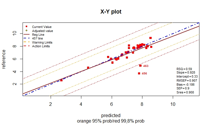
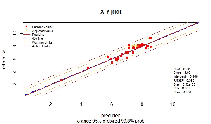
#' For Moisture and Fat there is an improvement using the model
#' with MSC math treatment,
#' For Protein the result are almost the same, but with the
#' raw spectra the is a certain slope and intercept problem,
#' and if corrected there is an improvement in the statistics.

PC Regressions with CARET

I did started to use Caret, and I will continue using it, so I have to try a lot of things in R to become familiar with it.

 

In Caret the are a data set (data=tecator) from a Tecator instrument for meat analysis, working in transmitance and in the range from 850 to 1050 nm with a total of 100 data points.

 

The parameters are Moisture, Fat and Protein. You can play around with this data to become familiar with Caret, so I try to create a quick regression with PCR.

 

Caret let us prepare the Training and Testing Data in a random order and to train the model with several kinds of cross validations. So I wrote some code apart from the help I found in the available Caret Documentation.

data(tecator)
set.seed(930)
colnames(absorp) <- paste("x", 1:ncol(absorp))
## We will model the protein content data
trainMeats <- createDataPartition(endpoints[,3], p = 3/4)
absorpTrain  <- absorp[trainMeats[[1]], ]
proteinTrain <- endpoints[trainMeats[[1]], 3]
absorpTest   <- absorp[-trainMeats[[1]], ]
proteinTest  <- endpoints[-trainMeats[[1]], 3]
trainData<-cbind(proteinTrain,absorpTrain)
testData<-cbind(proteinTest,absorpTest)
model <- train(proteinTrain~.,data=trainData, method = "pcr",
               scale = TRUE,
               trControl = trainControl("cv", number = 10),
               tuneLength = 10)
names(model)
model$bestTune
summary(model$finalModel)
predictions <- predict(model,testData)
plot(predictions,proteinTest)

With this code we get plots and statistics. This is my first step into Caret, where I would like to go really deep into. So I hope to write more posts about this subjet.

Monitoring Validations (Case 001)

I use R regularly for study the validations of different equations, in this case is an equation of cereals which include (barley, wheat, rye, corn, oat, triticale, ..). The monitor function in this case compare the starch values of an instrument consider as the Master (Y axis) and other consider as the Host (X axis).

 

The idea is to check if there are  differences which are important in order to take an action to adjust Bias or Slope and Intercept, or also consider to standardize the instruments.

 

In this case the Monitor function gives a warning to check if there are groups or extreme samples which can recommends the adjustment of slope and intercept.

 

 

And really there is a gap with two groups of samples, so we have to consider in this case what is happening: We have a group of barley samples with lower values of starch and a group with the wheat and corn samples with higher starch values.

 

In order to evaluate better we have to make subsets and check what is going on with the predictions statistics by groups and proceed the best way.

 



Comparing Posteriors: Estimating Practical Differences Between Models

Is not the first time Max Kuhn appears in this blog and this time with a lecture (in the last New York R Conference) about advices to estimate what is the best model based on R statistics. Sure we can get good advices  to find the best model possible for our data sets.

2018 New York R Conference Highlights

On April 20 this year the New York R Conference has been celebrated with a great  success.
Just look to the great atmosphere in the video of the conference.

Checking the slopes in Validation Groups

This is an study to develop calibrations for meat in a reflectance instrument from 1100 to 1650 nm. Normally meat are measured in transmitance but this is an approach to do it in reflectance.

 

I have just 64 samples with fat laboratory data. I split the spectra into 4 sets of 16 samples and merge 3 of leaving the other three for external validation. So I have 48 samples for training and 16 for validation and I can develop four calibrations and validate with 4 external sets.

 

Considering that we have few samples are in the training set, I have to use few terms. The SEPs for external or Cross Validation are quite high , but the idea here is to see the changes in the slope for the four validation sets.

 

The reason is that we have few samples and the slope value will stabilize as soon as more samples are included into the calibration and validation sets.

 

 

 

To improve the SEP we have to check the sample presentation method for this product and the procedure to obtain the laboratory reference method.

Monitoring the performance with the histogram

NIR can be used to detect levels food additives and check if they are in the right limits.

In this cases there are several types of doughs, and they use two levels of additive concentration depending on the type. So we have always the same reference data.

A calibration is developed and we have new data to validate. NIR will give  results which I expect to be covering the reference value with a Gauss distribution.

Using the Monitor function I can see the prediction distribution vs. the reference distribution and check if the expectations are fine.

 

In the case of the higher concentration is fine, and in the lower concentration is skewed (that is why the S/I adjust is suggested).This can be a first approach to continue with this application with mor accurate reference values.

Are you R Curious? (** This is a FREE tutorial.) - Part 1

R for AI developers

R for AI developers: David Smith makes the case for R as a platform for developing models for intelligent applications, offering a few examples with details in the accompanying interactive code lab.

Validating Resemble Model with Monitor function

Continuing with this post evaluating the LOCAL model developed in Resemble. This time I use the Monitor function (one of the Monitor functions I am developing).

I create different subsets from the validation sample set for the different categories, In this case is for one time of puppies, and I am evaluating the moisture content. We can see that there are two outliers that increase the SEP, so we have to see if we remove this samples for some reasons.

Let´s validate first with this type of puppy subset and check the statistics:

> val1.moi.pup1<-subset(val1.moi,ID1u_moi=="PUPPY-1")
> val1.moi.pup1<-cbind.data.frame(val1.moi.pup1$Sample.u_moi, 
+                                 val1.moi.pup1$Yu_moi, 
+                                 val1.moi.pup1$predicted.moi.local)

 

> monitor10c24xyplot(val1.moi.pup1)

Samples with the Sample IDs 463 y 456 are out of the action limits and the monitor function shows their position in the table:

$ResWarning [1] id ref pred res <0 rows> (or 0-length row.names) $ResAction id ref pred res 34 456 3.7 7.793351 -4.093351 32 463 4.9 7.881543 -2.981543

Now we can remove this samples knowing their position and recalculate:
val1.moi.pup1<-val1.moi.pup1[-c(32,34),]
monitor10c24xyplot(val1.moi.pup1)

Plots in Resemble (part 2)

Good results for the prediction of the validation samples (Xu, Yu) for protein. This is the XY plot where we can see in different colors the classes of the validation samples (different types of petfood). the SEP is 0.88 (without removing outliers) . Defining the data frame by classes will allow us to see the SEP for every class so we can check which class needs for more samples in the training database (Xr, Yr) or to check for other reasons.

plot(predicted.local,Yu_prot,col=val1.prot$ID1u_prot,lwd=2)

El error SEP de las muestras de validación de proteína es   :  0.887 

El R cuadrado para las muestras de validación de proteína es:  0.962 

 

 

Plots in Resemble (Part 1)

Resemble allow a certain number of plots which are very useful for your works or personal papers. In this case I use the same sets than of the previous post and I plot the PCA scores, where I can see the training matrix (Xr) scores and the validation matrix (Xu) scores overlapped.

 

Validation set is a 35% (randomly selected) of the whole sample population obtained from a long time period.

 

We can see how the validation samples cover more or less the space of the training samples.

> par(mfrow=c(1,2))
> plot(local.mbl, g = "pca", pcs=c(1,2)) 
> plot(local.mbl, g = "pca", pcs=c(1,3))

 

Using correlation in LOCAL (Resemble package)

> ctrl.mbl <- mblControl(sm = "cor",

                  pcSelection = list("cumvar", 0.999),
                  valMethod = "NNv",
                  scaled = FALSE, center = TRUE)

 > local.mbl <- mbl(Yr = Yr, Xr = Xr, Yu = Yu, Xu = Xu,

mblCtrl = ctrl.mbl,

                   dissUsage = "none",

                   k = seq(40, 150, by = 10),

                   pls.c = c(5, 15),

                   method = "wapls1")

 

Predicting sample: 1  ----------
Predicting sample: 2  ----------
Predicting sample: 3  ----------
Predicting sample: 4  ----------
Predicting sample: 5  ----------

--------------------------------

--------------------------------

> plot(predicted.local,Yu)

  

 

 

This time I use correlation (as Win ISI use) and try to find the best number of samples to select for the LOCAL algorithm with a sequence. 

As we can see the predictions improve with more samples in the calibration (red dots), maybe could be better win more samples by at the end of the plot it start to stabilize.

 

 

 

 

 

LOCAL Calibrations with Resemble

Really interesting the Resemble package so I am trying to work and understand it better even to help me in the case of Win ISI LOCAL calibrations.

We can get predictions for different combinations of local selected samples for the calibration to predict the unknown, so we can see the best option. We use a certain number of terms (min. and max.) and a weighted average  is calculated.

 

In this case I use an external validation set of petfood Xu with Reference data (protein) Yu, and I want to know the statistics (RMSE and R square) for the case of 90 local samples selected:

predicted.local <- as.numeric(Yu_anl$Nearest_neighbours_90)
> rmse.local <- sqrt(mean((Yu - predicted.local)^2))
> R2.local <- cor(Yu, predicted.local)^2
> R2.local
[1] 0.9507232
> rmse.local
[1] 1.163304

 

plot(predicted.local,Yu)

There are a lot of options to explore, so I will continue checking this package.

 

 

Memory based learning methods and tools (Resamble / LOCAL)

This is the link to this presentation which help us to understand the concept of LOCAL that we will treat during next posts with the "Resamble package" and we have treated and we will continue with LOCAL in Win ISI.

Developing LOCAL calibrations with R

We can use also LOCAL in R with the Resemble package. I am testing the package these days with a set of petfood spectra (with protein reference values) imported from Win ISI with SNV and a second derivative math treatment. After, I select 65% for training and the rest for test.

 

The get predictions process of Resemble allow a configuration to check for the better number of sample or factors for the better prediction, so there are a lot of options and functions to check in this package.

 

This is a plot of the results for a standard configuration from the reference manual, that I would try to go more deep into, trying to find the best configuration.

ctrl <- mblControl(sm = "pls",
                   pcSelection = list("opc", 40),
                   valMethod = c("NNv"),
                   scaled = FALSE, center = TRUE)

ex1 <- mbl(Yr = Yr, Xr = Xr, Yu = NULL, Xu = Xu,
           mblCtrl = ctrl,
           distUsage = "predictors",
           k = seq(30, 150, 15),
           method = "wapls1",
           pls.c= c(7, 20))
Yu_anl<-getPredictions(ex1)

Clearly seems that some of the configurations have overfitting, but I am just starting to learn the package so more post will come up giving my progress with this package.