Practice with Cereal Data (Chemometric package)

This is a post to follow the example of the cereal data in the book “Introduction to multivariate Statistical Analysis in Chemometrics” (Kurt Varmuza & Peter Filzmoser).

PLS2 is applied to a Cereal Data set with the function “mvr” using the cross validation “LOO: leave one out”.

The validation plot shows the error of the validation vs the number o PLS terms, for the different constituents.

A for every constituent the number of terms choose can be different, so an average is recommended.

This plot shows the error of the validation vs the number o PLS terms, for all the constituents overlapped.

As we can see, we choose 7 components for the model.

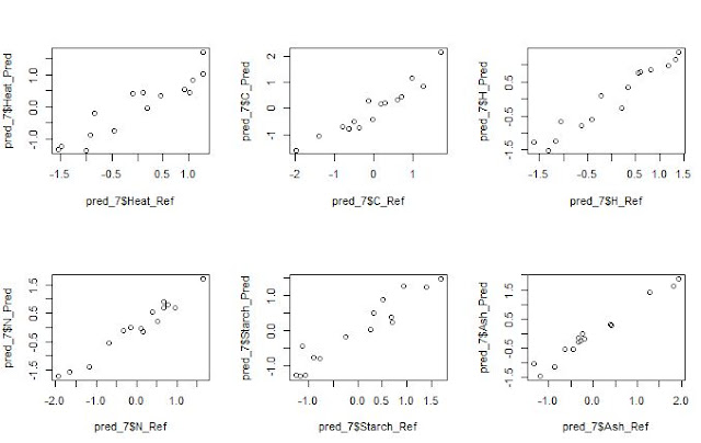
We can see the XY plots (reference vs predicted) with 7 terms for all the constituents.

pred7<-predict(respls2, cereal, ncomp = 7,type = c("response"))

par(mfrow=c(2,3))

     plot(pred_7$Heat_Ref,pred_7$Heat_Pred)

     plot(pred_7$C_Ref,pred_7$C_Pred)

     plot(pred_7$H_Ref,pred_7$H_Pred)

     plot(pred_7$N_Ref,pred_7$N_Pred)

     plot(pred_7$Starch_Ref,pred_7$Starch_Pred)

     plot(pred_7$Ash_Ref,pred_7$Ash_Pred)

Looking to the Residuals Plot.

Even if an application recommend us to make a type of adjustment, we have to look always to the plots.

In this case due to 3 samples (with prediction higher than 30) which are bellow the zero residual line, the application recommend us to adjust the slope, 

but it is clearly seen that for the rest of the samples the problem is a clear Bias problem. So we remove these samples with a prediction higher than 30 from the original data frame:

pass1<-subset(pass1$Table1,pass1$Table1[,3]<30)

and now the application will recommend the adjustment of the Bias. It is clear that we need more samples of this type in the plot to see clearly if we have a 

problem in the prediction of the protein content in this case.

The red dots are the sample values without bias adjustment and the yellow ones the samples with bias adjustments. The distribution of the yellow dots is fine 

and represents the random noise.

It is clear that more work must be done on the calibration or in the analysis of 

the reference methods in order to improve the predictions.

Validation Samples  = 85 
Reference Mean  = 21.7 
Predicted Mean  = 20.1 
RMSEP           : 2.35 (Current Error)
Bias            : 1.59 (Sugested Bias correction)
SEP             : 1.74 (Random error once Bias is corrected)

 

VIDEO: The Joy of Stats

Validation Report

Finally I was able to solve some issues with the data frames used in the monitor function, which converted the characters columns to factors so the sample identification was changed in case it contains not just numbers (as.is=TRUE will solve this problem). It was important also to extend the data frames correctly, this way the new data frame has the same structure all the time and everything worked fine.

The final report can be improved and new update could be added in the future, but at the moment quite happy with the results.

This could be a report for a protein validation in some kind of sausages measured by a NIT instrument and the reference method:

> monitor10c22dev(sausage,sortref=FALSE,eqalaxis=TRUE)
Validation Samples  = 88 
Reference Mean  = 22 
Predicted Mean  = 20.6 
RMSEP    : 2.49        (actual error)
Bias     : 1.39 
SEP      : 2.07        (error if we correct the Bias)
Corr     : 0.915 
RSQ      : 0.838 
Slope    : 0.884 
Intercept: 3.77 
RER      : 11.8   Poor 
RPD      : 2.46   Fair 
Residual Std Dev is : 2 (Error if we correct slope/intercept)
    ***Slope/Intercept adjustment is recommended***
BCL(+/-): 0.439 
    ***Bias adjustment in not necessary***
Without any adjustment and using  SEP as std dev the residual distibution is: 
  Residuals into 68%   prob (+/- 1SEP)    = 54     % = 61.4 
  Residuals into 95%   prob (+/- 2SEP)    = 83     % = 94.3 
  Residuals into 99.5% prob (+/- 3SEP)    = 87     % = 98.9 
  Residuals outside 99.5% prob (+/- 3SEP) = 1      % = 1.14 
With S/I correction and using Sres as standard deviation, the Residual Distribution would be:
  Residuals into 68%   prob (+/- 1Sres)     = 67     % = 76.1 
  Residuals into 95%   prob (+/- 2Sres)     = 84     % = 95.5 
  Residuals into 99.5% prob (+/- 3Sres)     = 87     % = 98.9 
  Residuals outside  99.5% prob (> 3Sres)   = 1      % = 1.14 

Adding statistic values to the X-Y plot

I was looking for the best way to add statistic values to the plot, and I found a way in this post  "Adding p values and R squared values to a plot using expression() ". It was really helpfull.
Just to check it I add the RSQ and Slope statistics, but the idea is to add more, so lloking to the plot you can have an idea about how the model performs.

Mixing in the Legends dots and lines

Finally I found the info to mix dot and lines in a plot, this way the plot looks nicer:
legend("topright",
        legend =c("Reg Line","Reg Line Bias Corr",
        "Current Value"","Bias adj. value"),
        bty = "n",
        col = c("brown","green4","red","black"),
        lty = c(1,1,0,0),                  
        lwd = c(2,2,0,0),                    
        pch = c(NA, NA, 15,21),           
        pt.bg = c(NA,NA,"red", "yellow"),
        pt.cex =0.5)

 

Looking to the Boxplots

Looking to the Boxplots can gives a quick idea of which of the different adjustments would work better. In this case the comparison is between the reference values, the predicted values corrected by the bias, the predicted values corrected by slope/intercept and the predicted values without any correction.
Boxplots help us as well to check the distribution and if there are outliers in the data sets.

Improving plots in the Monitor Function

I am trying to find the best way to check the performance of a model comparing the reference values with the predicted values and to see the efect of a bias adjustment, so after working on the function a plot is generated.
I will probably add two more plots, but I would not want to overcharge the plotted information.
I will see.
At the moment the info generated with the function is:

> monitor10c12(Muestra,HUM_NUT,HUM_ING,sortref=TRUE)
WARNING: More than 20 samples are needed to run the Validation 
Validation Samples  = 16 
RMSEP    : 0.742 
Bias     : -0.707 
SEP      : 0.233 
Corr     : 0.989 
RSQ      : 0.979 
Slope    : 0.907 
Intercept: 0.275 
RER      : 16.1   Fair 
RPD      : 6.17   Excellent 
BCL(+/-): 0.124 
      ***Bias adjustment is recommended***
Residual Std Dev is : 0.198 
    ***Slope adjustment is recommended***
Using  SEP as std dev the residual distibution is: 
  Residuals into 68%   prob (+/- 1SEP)    = 0     % = 0 
  Residuals into 95%   prob (+/- 2SEP)    = 3     % = 18.8 
  Residuals into 99.5% prob (+/- 3SEP)    = 7     % = 43.8 
  Residuals outside 99.5% prob (+/- 3SEP) = 9     % = 56.2 
  Samples outside UAL  = 0 
  Samples outside UWL  = 0 
  Samples inside   WL  = 3 
  Samples outside LWL  = 13 
  Samples outside LAL  = 9 
With Bias correction the Residual Distribution would be:
  Residuals into 68%   prob (+/- 1SEP)     = 13     % = 81.2 
  Residuals into 95%   prob (+/- 2SEP)     = 15     % = 93.8 
  Residuals into 99.5% prob (+/- 3SEP)     = 16     % = 100 
  Residuals outside  99.5% prob (> 3SEP)   = 0      % = 0 

Is my model performing as expected? (Part 2)

Really is true when whe say that a picture explain more than a thousand words, and this can be the case when I was trying to explain in the post "Is my model performing as expected? (Part 1)", the decission that a bias should be adjusted looking to the distribution statistics and errors.

But if we overplot the current residuals without adjustment (red dots), and the residuals with the adjustment (blue dots), we can see how the distribution moves into the warning limits.

plot(res~l,main="Residuals",ylim=c(-5*sep,5*sep),
     sub="orange 95% prob / red 99,8% prob",pch=15,col=2,
     xlab="sample position",ylab="residual")
abline(h=0,col="blue")
abline(h=(2*sep),col="orange")
abline(h=(-2*sep),col="orange")
abline(h=(3*sep),col="red")
abline(h=(-3*sep),col="red")
par(new=TRUE)
plot(Table2$res.corr1~l,col=3,ylim=c(-5*sep,5*sep),xlab="sample position",ylab="residual")

Is my model performing as expected? (Part 1)

 Hi all, I am quite busy so I have few time to expend on the blog, anyway I have continue working with R trying to develop functions  in order to check if our models perform as expected or not.

Residual plots and the limits (UAL,UWL,LWL,UAL) we draw on them will help us to take decisions, but developing some functions can help us to see suggestions in order to take good decisions.
So I am trying to works on this.

We always want to compare the results from a Host to a Master, the predicted NIR results with the Lab results,….

In all these predictions we have to provide realistic statistics and not too optimistic, if not we will not understand really how our model performs. Validation statistics, and looking to the residual plots will help us to understand if: our standardization is performing fine, if we have a bias problem or if the samples of the validation should be include in the data set and recalibrate again.

In this case is important to know the RMSEP of our calibration which can be the SECV for example (standard error of cross validation), and compare this error with the RMSEP of the validation, and after this with the SEP (validation error corrected by bias).
Is important to see how the samples are distributed in the residual plot into the warning limits (UWL and LWL) and into the action limits (UAL and LAL), are they distributes randomly?, do they have a bias?, if I correct the bias the distribution becomes random and into limits?,.....There are several questions that if we have the correct answer will help us to improve the model, and to
understand and explain to others the results we obtain.

This is a case where the model performs with a Bias:

Validation Samples  = 9

RMSEP    : 0.62

Bias     : -0.593

SEP      : 0.189

Corr     : 0.991

RSQ      : 0.983

Slope    : 0.928

Intercept: 0.111

RER      : 18.8   Fair

RPD      : 7.02   Excellent

BCL(+/-) : 0.143

***Bias adjustment is recommended***

The residual plot confirms that we have a bias:

Using SEP as std dev the residual distibution is:

  Residuals into 68%   prob (+/- 1SEP)    = 0

  Residuals into 95%   prob (+/- 2SEP)    = 1

  Residuals into 99.5% prob (+/- 3SEP)    = 4

  Residuals outside 99.5% prob (+/- 3SEP) = 5

  Samples outside UAL  = 0

  Samples outside UWL  = 0

  Samples inside   WL  = 1

  Samples outside LWL  = 8

  Samples outside LAL  = 5

With Bias correction the Residual Distribution would be:

  Residuals into 68%   prob (+/- 1SEP) =7

  Residuals into 95%   prob (+/- 2SEP) =9

  Residuals into 99.5% prob (+/- 3SEP) =9

  Residuals out  99.5% prob (> 3SEP)   =0

With the bias correction the statistics are better and confirm that probably a non robust standardization has been done with these two instruments that we are comparing.

This can help us to check other standardizations or decide if we need other algorithms as repeatibility file in the calibration or to mix spectra from both instruments.

RMS calculation in the Diagnostics

If you are use to work with ISI Scan, you can see a noise statistic summary for every cycle (totally 10) of the noise spectra, and two of those statistics are the bias and RMS.

Here I show the statistics for the first four cycles, but we only consider the NIR segment:

 

This post checks how ISI Scan calculates the RMS, and we can see that this RMS value is the RMS corrected by the Bias, so it tells us a measure of the random noise.

I show a simple script showing this:

cycle1<-noise[1,]
cycle2<-noise[2,]
cycle3<-noise[3,]
cycle4<-noise[4,]

 

options(digits=2)
rms1<-sqrt(mean((cycle1)^2)-(rowMeans(cycle1))^2)
rms2<-sqrt(mean((cycle2)^2)-(rowMeans(cycle2))^2)
rms3<-sqrt(mean((cycle3)^2)-(rowMeans(cycle3))^2)
rms4<-sqrt(mean((cycle4)^2)-(rowMeans(cycle4))^2)

> rms1
    1 
0.014 
> rms2
    2 
0.016 
> rms3
    3 
0.011 
> rms4
    4 
0.015 

Looking to the Residual Matrix

The first plot shows in blue color the residual Matrix "E", after developing a principal components calculation with SVD of some samples of wheat flour without any additive (training set).

Additive (ascorbic acid) was added to the flour in certain levels (50, 100, 200 and 500 ppm) to build a validation set. After acquiring the spectra, I reconstruct these spectra with the loading matrix "P" calculates with the SVD using the training samples. First I calculate the scores anf after the reconstructed spectra multiplying the scores with the P transpose matrix.

Once I get the reconstructed spectra, I subtract the reconstructed from the original validation set, and I get the residuals, that I overplot with red color over the blue ones.

I can see that the RMS is higher, and there is some shape different from the random noise of the blue spectra, so the good product model can be tuned to reject this validation set with some RMS cutoff.

Does this shape something from the spectra from the pure additive?

 

 

In green color we can see the spectra of the ascorbic acid, and I convert it into the residuals scale, and where I see certain similarities is in the band at 2250 nm, where all the peaks from the residuals of the validation set, and the ascorbic peak have the same shape.

Anyway this is a simply study about how residuals could help us to determine if the samples can be considered as Good Product, or they are out of specifications and further investigation is needed studying the residuals to determine the cause.

Artificial Check Cells (DS2500 and DA1650)

In order to have a stable check cell over time, manufacturers prepare samples more stable, but at the same time these samples are predicted by a model, and normally this model is not a robust one, so it is sensible to temperature, stabilization of the instrument, laboratory and instrument conditions.

A new generation of instruments like the DS2500 and DA1650 from Foss comes with an artificial Check Sample which contains a cake of Melamine and Talc. The distance between the cake and the window can vary slightly, so when scanning the Check Sample, you don´t have to look to the value of the subsamples for the parameter called Distance, if not to the average value.

The Distance value uses a formula, which contains 5 different properties of the average spectra.

The distance value will change depending of the temperature, so it is important to scan it when the instrument is fully warm up, and also the lab conditions. It is not recommended to keep in the Check Sample History, scans at different conditions.

Check Sample Definition must be redefined after Instrument calibration or lamp replacement.

“Be aware that the artificial check sample cell is just for instrument monitoring. The can indicate that something is going on that needs investigating but seldom alone justify a corrective action” (FOSS advice).