

4 feb 2012
"R": PLS Regression (Gasoline) - 003
The gasoline data set has the spectra of 60 samples acquired by diffuse reflectance from 900 to 1700 nm. We saw how to plot the spectra in the previous post.
Now, following the tutorial of Bjorn-Helge Mevik published in "R-News Volume 6/3, August 2006", we will do the PLS regression:
gas1 <- plsr(octane~NIR, ncomp = 10,data = gasoline, validation = "LOO")
This will fit a model of 10 components.
We will use the "Leave one out Cross Validation" (LOO)
The constituent is the octane number.
> summary(gas1)
Data: X dimension: 60 401
Y dimension: 60 1
Fit method: kernelpls
Number of components considered: 10
VALIDATION: RMSEP
Cross-validated using 60 leave-one-out segments.
(Intercept) 1 comps 2 comps 3 comps 4 comps 5 comps 6 comps
CV 1.543 1.328 0.3813 0.2579 0.2412 0.2412 0.2294
adjCV 1.543 1.328 0.3793 0.2577 0.2410 0.2405 0.2288
7 comps 8 comps 9 comps 10 comps
CV 0.2191 0.2280 0.2422 0.2441
adjCV 0.2183 0.2273 0.2411 0.2433
TRAINING: % variance explained
1 comps 2 comps 3 comps 4 comps 5 comps 6 comps 7 comps 8 comps
X 70.97 78.56 86.15 95.40 96.12 96.97 97.32 98.10
octane 31.90 94.66 97.71 98.01 98.68 98.93 99.06 99.11
9 comps 10 comps
X 98.32 98.71
octane 99.20 99.24
One way to decide better the number of components to use, is to plot the RMSEPs:
> plot(RMSEP(gas1), legendpos = "topright")

adjCV is the RMSEP Bias corrected which in the case of "LOO" is almost the same that the RMSEP without correction.
The plot suggest three components giving a RMSEP of 0.258.
Now we can see the different plots like the prediction plot:
> plot(gas1, ncomp = 3, asp = 1, line = TRUE)

We will continue with more plots in the next post.
Tutorials of :
Bjorn-Helge Mevik
Norwegian University of Life Sciences
Ron Wehrens
Radboud University NijmegenTweet
2 feb 2012
"R": Plotting the spectra (Gasoline) - 002
"R" has a package called "ChemometricsWithR", where we can get data from different analytical instruments including Near Infrared (NIR).
Follow the steps to plot the spectra of a gasoline data set:
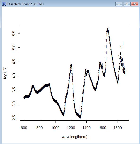
In this other case we plot the spectra of the NIR shootout 2002:

Tweet
Follow the steps to plot the spectra of a gasoline data set:
In this other case we plot the spectra of the NIR shootout 2002:
> data(shootout)
> wavelengths<-seq(600, 1898,by=2)
> mattplot(wavelengths,shootout$calibrate.1[1,],xlab="wavelength(nm)",ylab="log1/R)")
> library(ChemometricsWithR)
> data(gasoline, package="pls")
> wavelengths<-seq(900, 1700,by=2)
> matplot(wavelengths,t(gasoline$NIR),lty=1,xlab="wavelengths(nm)",ylab="log(1/R)")

Tweet
1 feb 2012
"R": Looking at the Data (Gasoline) - 001
As other softwares "R" has nice tools to look to the data before to develop the calibration.
Statistics for the "Y" variable (in this case octane number) like Maximun, Minimun,..,standard deviation,...are important:

Tutorials of :
Bjorn-Helge Mevik
Tweet
Statistics for the "Y" variable (in this case octane number) like Maximun, Minimun,..,standard deviation,...are important:
> library(ChemometricsWithR)
> data(gasoline)
> summary(gasoline$octane)
Min. 1st Qu. Median Mean 3rd Qu. Max.
83.40 85.88 87.75 87.18 88.45 89.60
> sd(gasoline$octane)
[1] 1.530078
And of course the Histogram:> hist(gasoline$octane)

Bibliography:
Tutorials of :
Bjorn-Helge Mevik
Norwegian University of Life Sciences
Ron Wehrens
Radboud University NijmegenTweet
30 ene 2012
Updating the equation
We have new data to update the calibration for a pet food category.
This data comes has been kept from different validations, and we decide that is time to update the calibration from different reasons (we have new variability: new batches, new formulation,….).
After looking at the spectra (searching for X outliers).We divide again the data set into validation and calibration sets, an develop different calibrations for each constituents in search of the best math treatment, more or less terms,….., which treatment take out less outliers, which more,….
Take notes, find answers and conclusions:
This is an example for the protein:

Important to look at the SEV (standard error of validation) we get for the Validation Set chosen randomly, and the other statistics.
Think that in a normal case:
SEC < SECV < SEV
After this study, mix again validation and calibration samples and develop the calibration (for each constituent) with the settings you found better. Probably this option increase change the number of terms, and of course will change the statistics.
After this study, mix again validation and calibration samples and develop the calibration (for each constituent) with the settings you found better. Probably this option increase change the number of terms, and of course will change the statistics.
After all the calibrations are developed, compare the new statistics with the ones of the previous equations.
Statistics can improve or even to be worse. Think why:
Look at the Mean and Std. Dev.
In this case I´m quite happy because I got a good improvement in the ash constituent. But the others have new variability and more samples and that is also very important.

Install the calibration in routine, and store new samples for the next validation.
Make a control chart (residual vs. lab value) meanwhile to control the calibration.
Tweet
Suscribirse a:
Entradas (Atom)