This was useR!2017 - Use R 2018 is coming

 

Registration and talk proposals open Monday for useR!2018

Trying to understand the regression coefficients

When developing the regression protein in R, one of the values obtained are the regression coefficients which are used to calculate the protein value for every new sample. There is a regression coefficient for every wavelength, so we can make a plot for the regression coefficients which maybe help us to understand how the calibration is working, but is not always like this and sometimes are very difficult to understand or almost impossible.

In the case of the regression make (with 4 terms) for the soy meal in transmittance, we can see the coefficient values like this.

attach(Prot_plsr_r1)
coefficients[,,4]
wavelengths<-as.matrix(seq(850,1048,by=2))
matplot(wavelengths,coefficients[,,4],type="l",
        xlab="wavelengths",ylab="coefficients")

We can look for the peaks:

library(quantmod)
findPeaks(coefficients[,,4])

 

The results are that we have peaks at:

 

soy_ift_prot1r1$X_msc.....880nm  (Starch band)

 

soy_ift_prot1r1$X_msc.....910nm  (Protein band)

 

soy_ift_prot1r1$X_msc.....968nm  (Fat band)

soy_ift_prot1r1$X_msc....1028nm  (Protein / Fat band)                       

The results make some sense and make me a little more confident that the regression will work fine in routine.

 

Analyzing soy meal in transmittance (part 10 and last)

This is the last post about analyzing soy meal in transmittance. The last option we make was to make a special selection from the original database to see if we get some improvements in the performance of the calibration, but with this option appears some slope, so I prefer the first option were the statistics were quite good but with a Bias.

With all the database the statistics for the PLS regression (with 4 terms) are:
RMSEP..........1,12
SEP............0,529  (Prediction error bias corrected)
RSQ............0,898
and the XY plot is:

With the samples selected with the approach described in the part 9, the statistics are:
RMSEP.......1,12
SEP.........0,633  (Prediction error bias corrected)
Sres........0,547 (Prediction error Slope/Intercept corrected)
RSQ.........0,898
and the XY plot is:

As we can see the first option is the best, and gives quite aceptable errors for protein in intact soy meal in transmittance.

 

And what about if we calibrate with Win ISI

 and validate with a model with the 5 terms in Win ISI:

Samples used for Statistics           27
Slope                                  0.871
Intercept                              5.283
Bias                                  -0.703
SEP                                    0.927
SEP(C)                                 0.616 (Bias corrected)
RSQ                                    0.864

as we can see there are some differences, but the statistics are quite similar and again we have a bias, and an acceptable error.

As a first step we can work with the model adjusted until new samples from the new instrument, be added to the database an the model is recalculated. 

 

Hope you all these posts and let me know if you need more details in the comments.

Analyzing soy meal in transmittance (part 9)

Analyzing soy meal in transmittance (part 8)

Analyzing soy meal in transmittance (part 7)

Analyzing soy meal in transmittance (part 6)

Analyzing soy meal in transmittance (part 5)

Analyzing soy meal in transmittance (part 4)

Analyzing soy meal in transmittance (part 3)

Analyzing soy meal in transmittance (part 2)

Analyzing soy meal in transmittance (part 1)

Analyzing Soy meal in transmittance (part 9)

In the case of the Soy meal, we have a validation sample set (from an Infratec Nova), and we get the predictions from a calibration sample set from an Infratec  1241. As we saw in "Analyzing Soy meal in transmittance (part 8)" , the predictions are fine, but we have a bias and the idea was to merge the samples from the Infratec Nova with the samples from the Infratec 1241 and to develop a calibration.

But before that we want to see another option, and for that we are going to use an option from Win ISI: "Select local samples from a product file".

With this option we project the validation samples in the PC space we got from the calibration samples, and we search for neighbors into a certain cutoff.

Those samples will be take them apart into a file, to develop an exclusive calibration for the validation samples.

In this case I am going to use a cutoff of 0,2 (Mahalanobis distance).

From the 657 samples, 527 were selected  and exported to R to develop the calibration. There are some clear outliers, but there is a high improve in the statistics.

Now we remove the samples with number in red, because they are out of the action limits and recalculate.

>soy_ift_prot_sel1_r1<-soy_ift_prot_sel1[-c(495,102,83,270,74),]

>Prot_plsr_sel_r1<-plsr(soy_ift_prot_sel1$Prot~soy_ift_prot_sel1   $Xsel_msc,ncomp=16,data=soy_ift_prot_sel1,validation = "LOO")

>predictions_sel_r1<-(Prot_plsr_sel_r1$fitted.values[,,9])
>soy_ift_prot_sel2_r1<-cbind(soy_ift_prot_sel1_r1$Sample,soy_ift_prot_sel1_r1$Prot,predictions_sel_r1)

>monitor_prot_sel<-monitor10c24xyplot(soy_ift_prot_sel2_r1)

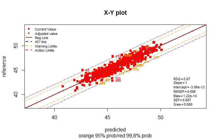
 As you can see there is an improvement in the calibration statistics with this selection, but is it an improvement in the validation. We will see it in the next post.

 

Analyzing Soy meal in transmittance (part 8)

Continuing from the post "Analyzing Soy meal in transmittance (part 7)", we are going to remove the four samples which are out of the action limit (residual higher than 3.RMSEP) , and to recalculate the model.
soy_ift_prot1r1<-soy_ift_prot1[-c(183,107,108,267),]
Prot_plsr_r1<- plsr(soy_ift_prot1r1$Prot~soy_ift_prot1r1$X_msc,
                    ncomp = 16,data =soy_ift_prot1,
                    validation = "LOO")
summary(Prot_plsr_r1)
predictions<-(Prot_plsr_r1$fitted.values[,,9])
soy_ift_prot2r1<-cbind(soy_ift_prot1r1$Sample,
                       soy_ift_prot1r1$Prot,
                       predictions)
monitor_prot_r1<-monitor10c24xyplot(soy_ift_prot2r1)
With this code we get the new X-Y plot and the new statistics, and finally we are going to keep this model.


I don´t consider necessary to remove more samples, and the Monitor function give us the distribution of the residuals into the different regions:

  Residuals into 68% prob (+/- 1SEP) = 459 % = 70.72419 Residuals into 95% prob (+/- 2SEP) = 611 % = 94.14484 Residuals into 99.5% prob (+/- 3SEP) = 646 % = 99.53775 Residuals outside 99.5% prob (+/- 3SEP) = 3    % = 0.4622496

 

As we can see we get a Gaussian distribution for the residuals.

 

This calibration was done with data from an IFT1241.There is a new instrument called Infratec NOVA, and an exercise has been done in order to check if the calibration developed in an Infratec 1241 can be used in routine in an Infratec NOVA. With this purpose a set of external validation samples had been analyzed in an Infratec NOVA using the same transmittance path length than in the Infratec.

Once the samples had ben analyzed the spectra has been exported and as reference values we add the predicted values obtained in NIR reflectance instruments calibrated with values for the official reference methods.

 

We will use this data to check the model or adjust it if necessary. We can validate using different number of terms to see if the model is overfitted for this external data set, and we will se that this is the case and that the best  results are for 4 terms, but there is a bias due probably to dome differences in the instruments itself.

With 4 terms the validation (with the Monitor function) is:

 

We see the actual values in red, and that a Bias adjustment is recommended, so with the bias adjustment we would see the yellow dots.
As we can see we have a bias, but the error with the Bias corrected is quite good (SEP=0,529).
If we add more terms the statistics are not so good like this, so maybe the best option is to add this samples to the data base and recalibrate to add the new variability to the model.