Access to Statistics: The top 20 data visualisation tools

Access to Statistics: The top 20 data visualisation tools: The top 20 data visualisation tools | .net magazine 17th Sep 2012 | 09:17 From simple charts to complex maps and infographics, Brian S...

Reference Standardization Concept

Vision has an option to import DA files (from NSAS ) into a project, so we import the file which comes with our standard set and we will see one file called R80xxxxx (the “x” are the serial number of the standards box set). This file is our Master Reference file.

If we acquire the spectra of this R80xxxxx in the Host instrument (our instrument), without reference standardization , the spectra is quite different to the Master spectra, so a Reference standardization is needed in order that the Master and the Host have in common the same reference spectra when acquiring a sample.

 

In the next picture we see the spectra of the R80xxxxx (Red in the Master and Blue in the Host without Ref STD).

 

We run the Reference standardization and a STD file is created to correct this differences from the Host to the Master. Other Hosts do the same and the idea of more transferable equations (between instruments) is possible because we are correcting most of the instruments differences.

Here we are not correcting wavelength shift, just photometric response.

There are standards sets with different ceramics in order to check the photometric response of the Host to the Master at different reflectance levels (R99xxxxx, R40xxxxx, R20xxxxx, R10xxxxx and R02xxxxx).

 

Let´s compare the R99xxxxx passed in the Host instrument with and without Reference Std.

 

Without Ref Std:





 

With Ref Std:

 

 

 

 

Sunflower seed Regressions with "R" - 001

I have spectra from sunflower seed grinded from 3 NIR instruments (range 400-2500 nm). I prepare the data frame separating the spectral range in two segments (Segment 1 or VIS from 400-1100 nm, and segment 2 or NIR from 1100 to 2500). Reference values are from four different laboratories.
 

In a previous post I have transformed the NIR raw spectra to MSC, using a function from the R package "Chemometrics with R".
 

In this post I want to run a regression with PLS (PLSR) using the Segment 2, and with the math treatment MSC.

sflw1 <- plsr(G00rmn~NIRmsc, ncomp = 10,data =sflw.msc2 ,
        validation = "LOO")

VALIDATION: RMSEP
Cross-validated using 107 leave-one-out segments.
      
          (Intercept)  1 comps  2 comps  3 comps   4 comps   5 comps  6 comps

CV           2.87         2.465       2.074      1.112      1.038     0.9903     0.9833
adjCV      2.87         2.465       2.074      1.111      1.038     0.9899     0.9829

                         7 comps  8 comps  9 comps  10 comps
CV                     0.9746     0.9781    0.9754    0.9683
adjCV                0.9741     0.9775    0.9745    0.9675


 TRAINING: % variance explained

              1 comps  2 comps  3 comps  4 comps  5 comps  6 comps  7 comps  8 comps
X              41.93     89.86       95.78      97.02      98.21      99.21      99.62      99.76
G00rmn    31.47     51.80       86.47      89.14      90.36      90.64      91.01      91.42

              9 comps  10 comps
X              99.81     99.89
G00rmn    92.30     92.62

 

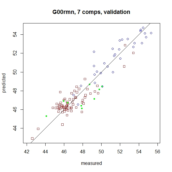
And now we can see the X-Y plot for the LOO Regression (with 7 comps), with different colors and symbols for the samples from the different instruments.

plot(sflw1, ncomp = 7, asp = 1, line = TRUE,

pch=c(20:22)[sflw.msc2$Operator],
col=c("green","blue","brown")[sflw.msc2$Operator])

 

 

Postcards from Asturias

Some days of hollidays this Easter to spend in Asturias. Up is a picture I take in  Lastres.
Down another nice village "Cudillero". 
Wish to all this Blog readers a nice Easter time.

Desearos a todos los lectores de este blog unos felices días de Semana Santa. Yo los he aprovechado para venir a Asturias.
En la foto superior os muestro Lastres, famoso poblado marinero,  debajo una foto de Cudillero.

Generating PDF docs with "R"

It is really amazing how while you are reading papers, bibliography,...., from the R community, how you can apply all these knowledge´s to your work in order to prepare nice documents.
In this plot you can see the spectra from sunflower seed without any treatment in the first column, and treated with MSC in the second (to remove scatter).

This plot has been generated in a PDF document with the script:

pdf("fig-1-1.pdf",width=9,height=7)
par(mfrow=c(3,2),mar=c(4,4,3,3))

Now we add all the plot script:

matplot(wave.ALL,t(ALL),type="l",lty=1,xlab="nm",
      ylab="log 1/R",col="blue",main="Sunflower RAW Spectra")
matplot(wave.VIS,t(VIS),type="l",lty=1,xlab="nm",
      ylab="log 1/R",col="blue",main="Sunflower RAW Spectra")
matplot(wave.NIR,t(NIR),type="l",lty=1,xlab="nm",
        ylab="log 1/R",col="blue",main="Sunflower RAW Spectra")
matplot(wave.ALL,t(ALLmsc),type="l",lty=1,xlab="nm",
ylab="log 1/R",col="blue",main="SFLW Spec MSC")
matplot(wave.VIS,t(VISmsc),type="l",lty=1,xlab="nm",
        ylab="log 1/R",col="blue",main="VIS segment SFLW Spec with MSC")
matplot(wave.NIR,t(NIRmsc),type="l",lty=1,xlab="nm",
        ylab="log 1/R",col="blue",main="NIR segment SFLW Spec with MSC")

and we finish with:

dev.off()

I use in this case for the documents the same settings than