Working with Soilspec data (part 9)

Once we split the soilspec data into the selected samples (pu$model) and the others (samples non selected  pu$test), we can take them apart with our favorite math treatment (in this case SNV and Detrend):

pu_sel<- spectra_snvdt[pu$model,]
pu_nonsel<- spectra_snvdt[ pu$test,]
matplot(as.numeric(colnames(pu_sel)),t(pu_sel),type = "l",
        col = "blue", xlab = "wavelength", 

        ylab = "Log 1/R")
par(new=TRUE)
matplot(as.numeric(colnames(pu_nonsel)), t(pu_nonsel), 

        type = "l",
        col = "red", xlab = " ", ylab = " ")

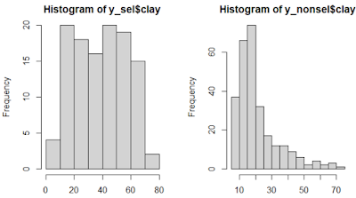
We can do the same for the "Y" matrix with the parameters, and look to one of the histograms (for clay for example):

y_sel<- parameters[pu$model, ]

y_nonsel<- parameters[pu$test, ]

par(mfrow = c(1,2))

hist(y_sel$clay)

hist(y_nonsel$clay)

Now we have a group of samples (the selected ones) to develop the regressions, and we will use the non selected for validation.