Regression planes in R (wavelength space)

We have seen the high correlation between wavelengths in previous posts and how we can reduce the wavelength space from lower dimension plots. 

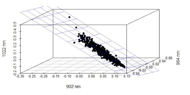
In the case of the 3 wavelengths selected in the previous post at 1022, 964 and 902 nm. 

We can use the wavelength at 1022 nm as the dependent variable and to calculate a MLR regresión to predict the absorbances at this wavelength as a linear combination of the absorbances at 902 and 964 nm calculating a regression plane;
    #1022nm     datapoint 87    
  # 902nm     datapoint 27  
  # 964nm     datapoint 58   
x1<-X_msc_mc[,c(27)]  
x2<-X_msc_mc[,c(58)]  
x3<-X_msc_mc[,c(87)]  
s3d<-scatterplot3d(x1,x2,x3,pch=16,highlight.3d = TRUE,
                   angle=330,xlab="902 nm",
                   ylab="964 nm",zlab="1022 nm")       
fit<-lm(x3~x1+x2)
s3d$plane3d(fit,lty.box = "solid")

We can see the plane looking to the new regression plane plot:

 

x1new=-1.170e-16+(-2.122e+00*x1) 
x2new=-1.170e-16+(-1.061e+00*x2) 
#plot(x1new,x2new)
x12new<-cbind(x1new,x2new)
library(chemometrics)
drawMahal(x12new,center=apply(x12new,2,mean),
          covariance=cov(x12new),quantile=0.975,col="blue")