Analazing Soy meal in transmitance (part 7)

In the values of the constituents, we have some values with zeros, so these values must not be considered during the calibration. If we have a long data set we can look for the minimum and maximum values, and if the minimum is zero we can remove the samples with this value to develop the quantitative models.

Here are the histograms of the data sets without the samples with zeros.

We can make a PLS regression with all the samples and after to remove the outliers we found clear. So for the protein the PLS regression would be:

Prot_plsr<- plsr(soy_ift_prot1$Prot~soy_ift_prot1$X_msc,
                 ncomp = 16,data =soy_ift_prot1,
                 validation = "LOO")

where we use the LOO (leave one out) validation.

The LOO cross validation, will help us to decide which is the best number of terms to choose for the regression, so we can look to one of the explained variance plot, where we can see how the RMSEP decrease as the number of terms increase, but there will be a certain number of PLS terms where the RMSEP stay stable or even increase, so we must nor choose more terms than necessary in order not to over fit the model.

plot(Prot_plsr,"validation",estimate="CV")

If we look to the regression summary,

summary(Prot_plsr)

we can see that the best number of terms for the regression is nine.

Let´s see the statistics in a XY plot, and for it I am going to use a Monitor function I developed in R some time ago.

predictions<-(Prot_plsr$fitted.values[,,7])

soy_ift_prot2<-cbind(soy_ift_prot1$Sample,

                     soy_ift_prot1$Prot,

                     predictions)
monitor10c24xyplot(soy_ift_prot2)

As we can see we must remove some outliers, which are out of the action limit (numbers in red), and decide what to do with the samples are out of the warning limit (numbers in orange).

The Monitor function take apart those sample, so we can remove them from the data frame and recalculate.

 

White paper about Artificial Neural Networks

White paper:

Artificial Neural Networks and Near Infrared Spectroscopy - A case study on protein content in whole wheat grain

Quantitative quick view (Soy meal analyzed in transmitance)

During this tutorial about the analysis of Soy meal in transmitance with an Infratec, we will see also the quantitative analysis, once we have seen the spectra characteristics.

This is just a quick look to a quantitative analysis to see where the extreme spectra samples appear in the XY plots of the quantitative analysis.

As we can see in some of the plots appear the sample "298" as an outlier (specially in Moisture). There are clearly chemical outliers with a high residual, due probably, to a mistake in the lab value.

Soy meal is normally analyzed by NIR instruments and not by NIT instruments, but we will continue with this work to see what statistics we can obtain from the equations and from a validation.

Analyzing Soy meal in transmitance (part 6)

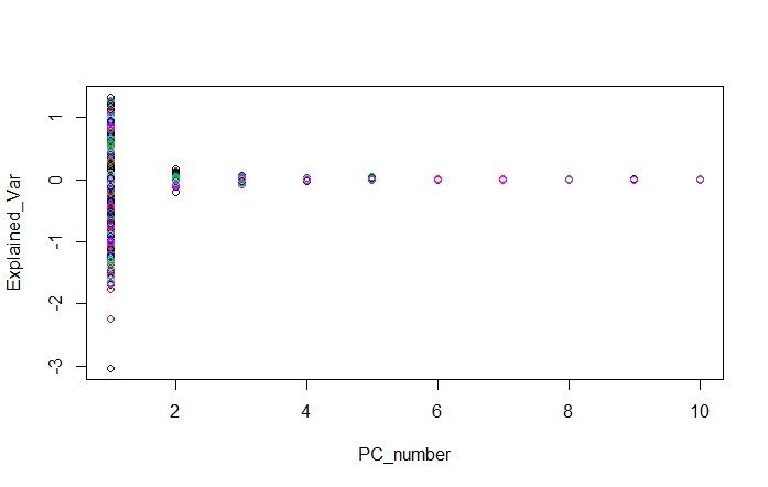
A good way to see the variance explained by the PCs is a 2D plot, where we see the projection of the scores over the PC terms, so it is a way to see in which PC term we can see a discrimination, or outliers.
In the case of the soy meal data, we can see the distribution of the scores in the plane formed by the first and second principal components.

 

and now imagine projecting the dots o perpendicularly over the axes (PCs), and this projections are the perpendicular dots of the next plot for the first and second PCs. In the projections of the first PC we see clearly out the samples 298 and 296, and if we would make a zoom of the second PC projections we would see clearly out the samples 373 and 298.

 

As we can see in this plot the whole variance of the data is explained by the first three PCs.

Analyzing Soy meal in transmitance (Part 5)

Under all these post about Analyzing Soy meal in transmitance there is the excuse to work with "R" and to see a lot of chemometric functions which the available R packages offer.
So continuing with this this is the fifth post about it.

We are more use to see the Mahalanobis distance with ellipses, so let see the same as in the previous post  with the "drawMahal" function of the Chemometric package.
First we use the Nipals algorithm to calculate the score matrix T and the loading matrix P with the X matrix with the Math treatment MSC (Multiple Scatter Correction).
X_msc_nipals<-nipals(X_msc,a=2)
T_msc<-X_msc_nipals$T
P_msc<-X_msc_nipals$P
drawMahal(T_msc,center=apply(T_msc,2,mean),
          covariance=cov(T_msc),
          quantile=0.975,col="blue",
          xlab="PC1",ylab="PC2")
identify(T_msc)

 

As we can see we have the same outliers, but we see them in a different way.