ISI Scan: Linking a product to "two different types of PMs"

This video is the reply to one of the followers of this blog. Hope you like:



See also:
Configuring ISI Scan to work with LOCAL

Median absolute deviation

Median absolute deviation - Wikipedia, the free encyclopedia

   

This is a robust statistic to use indeed the standard deviation. You can see in this Wikipedia link details of the theory.

This post is just to see how we can use this statistic with R for the calculation of the Principal Components.

Using the R Library: pcaPP, we use the function:

PCAgrid (x, k = 2, method = c ("mad", "sd", "qn"),.............)

In this function, we select the method to use, beeing "mad", the default one. "X" is our spectral matrix, and "k" is the number of components to compute.

Doing this calculations, we get a matrix with the loadings, and another matrix with the scores, apart from other staistics and values.

To follow some rules let´s call P to our loading matrix, and T to our scores matrix.

library(pcaPP)

sflw.msc.rpc<-PCAgrid(sflw.msc$NIRmsc,k=4,scale=mad)

P<-sflw.msc.rpc$loadings

T<-sflw.msc.rpc$scores

pairs(T[,1:4],col=c("red","blue","green","brown")[sflw.msc$Set])

I can see the samples used in the calibration set in green color and other comming from diferent instruments in other colors, in order to study the patterns and to know better my database.

 

 Continue this post with: Detecting outliers (Mahalanobis)

 

 

Validating R-PLS Sunflower Seed Model (Part 01)

I have ten new sunflower seed samples, with laboratory data and I´m going to use them to validate the performance of a model developed in R with PLS:
Sunflower seed Regressions with "R" - 001

First, I  have a look to the spectra of the validation set (red spectra) compares with the training spectra (blue spectra), without any math treatment applied:

and after, with the MSC applied:

I see clearly some differences, but the idea is to check if the calibration is robust enough to predict the samples according to the statistics we got in the summary of the regression.
In the summary of Sunflower seed Regressions with "R" - 001 , we decide to use 7 terms for our predictions, so:

predict(sflw.g00rmn,ncomp=4,newdata=sflw.msc2.val)

                     G00rmn
171     46.25923
173     53.07202
176     53.48508
177     53.27027
178     46.05511
179     46.73826
180     50.95862
181     52.44956
182     47.59493
183     46.51557
The error is:

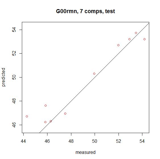
Let´s have a look to the "Reference vs Predicted" plot:

predplot(sflw.g00rmn,ncomp=7,newdata=sflw.msc3.val,
asp=1,line=TRUE,col=c("red"))

 

Transfering "oil / fat" Database - Transflectance

Today I have the task to transfer a oil/fat database from one instrument to other three instruments. Three of them are the same type and the other (where the database come from) has a different sample presentation (aluminum reflector), but all of them has the same sample presentation mode: "Transflectance".

 It is important to present the samples in the instruments at the same temperature.

Be careful that the sample covers the reflector without bubbles or gaps.

The gold reflectors are 0.1 mm, so the total path length is 0.2 mm. Anyway we must be careful because there are some minimum differences between them, and every instrument must use their respective reflector for the standardization.

These are the spectra of water acquired in the same instrument, but with three different gold reflectors of 0,1 mm.

 

LOCAL: Batch Mode to select Max Number of Samples

When working with LOCAL we have the choice to select the “Minimum Number of Samples” and the “Maximum Number of Samples” to develop the LOCAL calibration. This option can be done with the default option (where we can select the maximum and minimum values), or with the Batch mode where we select the Minimum and create a Batch for the Maximum (in this case 200, 250 and 300). We leave the software running this task and at the end we will get some statistics (SEP, RSQ, Bias…) and the Rank for the best choice for the “Maximum Number of Samples”.

I use a sample set with to check the best option with 213 values for moisture (HD), 238 for ash (CZ), 242 for fat (GB) and 235 for protein (PB).

The DataBase used is PetFood and in the validation set there was sample of different kinds of dogs and cats.

In this example the Best Choice is 300 samples so we can configure the Batch for more samples, just in case we get better statistics.

 

 

This is the Lab vs. Predicted plot (for the Validation Set), in the case of Fat (GB) selecting a maximun of 300 samples.