Practice with Cereal Data (Chemometric package)

This is a post to follow the example of the cereal data in the book “Introduction to multivariate Statistical Analysis in Chemometrics” (Kurt Varmuza & Peter Filzmoser).

PLS2 is applied to a Cereal Data set with the function “mvr” using the cross validation “LOO: leave one out”.

The validation plot shows the error of the validation vs the number o PLS terms, for the different constituents.

A for every constituent the number of terms choose can be different, so an average is recommended.

This plot shows the error of the validation vs the number o PLS terms, for all the constituents overlapped.

As we can see, we choose 7 components for the model.

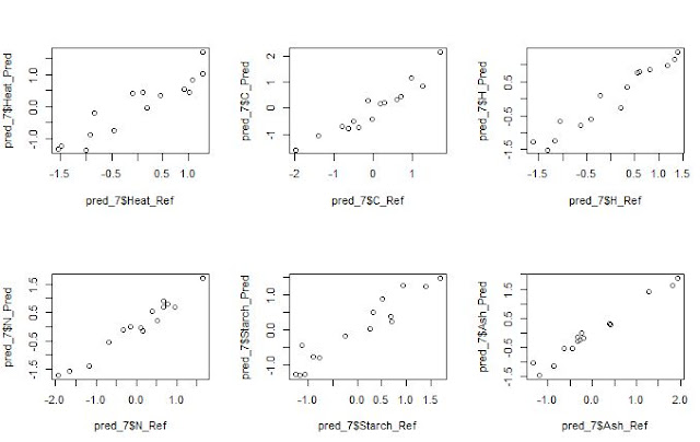
We can see the XY plots (reference vs predicted) with 7 terms for all the constituents.

pred7<-predict(respls2, cereal, ncomp = 7,type = c("response"))

par(mfrow=c(2,3))

     plot(pred_7$Heat_Ref,pred_7$Heat_Pred)

     plot(pred_7$C_Ref,pred_7$C_Pred)

     plot(pred_7$H_Ref,pred_7$H_Pred)

     plot(pred_7$N_Ref,pred_7$N_Pred)

     plot(pred_7$Starch_Ref,pred_7$Starch_Pred)

     plot(pred_7$Ash_Ref,pred_7$Ash_Pred)

Looking to the Residuals Plot.

Even if an application recommend us to make a type of adjustment, we have to look always to the plots.

In this case due to 3 samples (with prediction higher than 30) which are bellow the zero residual line, the application recommend us to adjust the slope, 

but it is clearly seen that for the rest of the samples the problem is a clear Bias problem. So we remove these samples with a prediction higher than 30 from the original data frame:

pass1<-subset(pass1$Table1,pass1$Table1[,3]<30)

and now the application will recommend the adjustment of the Bias. It is clear that we need more samples of this type in the plot to see clearly if we have a 

problem in the prediction of the protein content in this case.

The red dots are the sample values without bias adjustment and the yellow ones the samples with bias adjustments. The distribution of the yellow dots is fine 

and represents the random noise.

It is clear that more work must be done on the calibration or in the analysis of 

the reference methods in order to improve the predictions.

Validation Samples  = 85 
Reference Mean  = 21.7 
Predicted Mean  = 20.1 
RMSEP           : 2.35 (Current Error)
Bias            : 1.59 (Sugested Bias correction)
SEP             : 1.74 (Random error once Bias is corrected)

 

VIDEO: The Joy of Stats

Validation Report

Finally I was able to solve some issues with the data frames used in the monitor function, which converted the characters columns to factors so the sample identification was changed in case it contains not just numbers (as.is=TRUE will solve this problem). It was important also to extend the data frames correctly, this way the new data frame has the same structure all the time and everything worked fine.

The final report can be improved and new update could be added in the future, but at the moment quite happy with the results.

This could be a report for a protein validation in some kind of sausages measured by a NIT instrument and the reference method:

> monitor10c22dev(sausage,sortref=FALSE,eqalaxis=TRUE)
Validation Samples  = 88 
Reference Mean  = 22 
Predicted Mean  = 20.6 
RMSEP    : 2.49        (actual error)
Bias     : 1.39 
SEP      : 2.07        (error if we correct the Bias)
Corr     : 0.915 
RSQ      : 0.838 
Slope    : 0.884 
Intercept: 3.77 
RER      : 11.8   Poor 
RPD      : 2.46   Fair 
Residual Std Dev is : 2 (Error if we correct slope/intercept)
    ***Slope/Intercept adjustment is recommended***
BCL(+/-): 0.439 
    ***Bias adjustment in not necessary***
Without any adjustment and using  SEP as std dev the residual distibution is: 
  Residuals into 68%   prob (+/- 1SEP)    = 54     % = 61.4 
  Residuals into 95%   prob (+/- 2SEP)    = 83     % = 94.3 
  Residuals into 99.5% prob (+/- 3SEP)    = 87     % = 98.9 
  Residuals outside 99.5% prob (+/- 3SEP) = 1      % = 1.14 
With S/I correction and using Sres as standard deviation, the Residual Distribution would be:
  Residuals into 68%   prob (+/- 1Sres)     = 67     % = 76.1 
  Residuals into 95%   prob (+/- 2Sres)     = 84     % = 95.5 
  Residuals into 99.5% prob (+/- 3Sres)     = 87     % = 98.9 
  Residuals outside  99.5% prob (> 3Sres)   = 1      % = 1.14