Making things easier: Regression coefficients.

The idea of this post is: "Dont forget when you develop a regression, to look to the plots and try to interpret them".

Start making things easier. Sometimes easier things are more robust and stable.

Shootout 2012 : first PLS regressions

It´s time to start developing some regressions in order to find the best math treatment, the best number of terms, the best spectral regions, the best regression method,....

This time I´m working with the PLS  package in R, and just to make more familiarity with it, I us the pls regression, with the full range, and with two math treatments.: MSC and SG Filters (with first and second derivatives). I will try in other post to select spectral regions, or even other regression methods. 

Indeed to look to the Cross Validation statistics I will look to the prediction statistics for the test set. We have seen that the samples in this set are not fully represented by the training set, and if we predict them fine is a symptom that the equation is robust. Don´t forget that the idea is to predict as better as possible a validation set, which in theory we don´t know the values. (we already know them and I will compare my results in the future with the winner, and other participants).

I develop a regression (1) with MSC, and I look to the prediction statistics for the test set:
>Active_reg1<- pls(Active~NIT.msc,ncomp=5,data=shootcalmsc.2012 , validation = "LOO")
>RMSEP(Active_reg1,newdata=shoottestmsc.2012)

(Intercept)      1 comps      2 comps      3 comps      4 comps      5 comps 
     1.1637       0.6944       0.5028       0.4586       0.4913       0.5355

Now the regression (2) with a SG filter (first derivative)
>Active_reg2<- plsr(Active~NITsg, ncomp =5,data=shootcalsg.2012 , validation = "LOO")
>RMSEP(Active_reg2,newdata=shoottestmsc.2012)
(Intercept)      1 comps      2 comps      3 comps      4 comps      5 comps 
     1.1637       1.0414       0.4172       0.4313       0.4531       0.4556

In case that the SG filter has the second derivative, the RMSEP statistics are:
(Intercept)      1 comps      2 comps      3 comps      4 comps      5 comps 
     1.1637       0.5506       0.4269       0.4227       0.4134       0.4009

We can have a look to the Predicted vs. Lab plots:
>predplot(Active_reg1,ncomp=3,newdata=shoottestmsc.2012,asp=1,line=TRUE,main="MSC math-treatment")>predplot(Active_reg2,ncomp=2,newdata=shoottestsg.2012,asp=1,line=TRUE,main="SG second der")

Well, The plots are not really nice, It is clear that we can separate the two groups, but the results are not very accurate. I have to continue working on it in order to see if I improve this plot, looking to the RMSEP.

We can play with the parameters of the SG filter and try, but I think is better to select spectral regions. I will let you know in other post.

If you are interested in this post, there are some previous ones you can find also interesting:
"Sample Sets" plots (Shootout-2012)
Shootout 2012: Test & Val Sets proyections
Working with Shootout - 2012 in R (001)
Shootout 2012 files

Can NIR & Chemometrics be more accurate than the reference method?

Can NIR & Chemometrics be more accurate than the reference method?

In focus nº 2 -2012

A review of global ANN calibrations for whole grain analysis.

by:Robin Malm, Mark Westerhaus and Lars Nørgaard

VIDEO: Looking to the regression coefficients in R

Bonus:
There is another function to plot the regression coefficients: "coefplot"
I can use it in this case:
coefplot(Active_reg1, ncomp = 1:5,separate=TRUE)
to get this nice plot of the regression coefficients with one to five terms:

VIDEO: Looking to the loadings in R

Bonus:
You can use also this option:
plot(Active_reg1,"loadings",comps=1:3,legendpos="topleft")
to get this nice plot of the first three loadings:

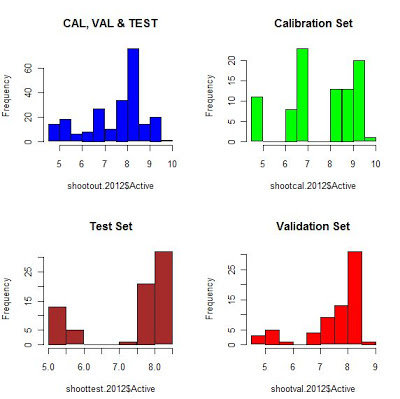
"Sample Sets" plots (Shootout-2012)

Histograms of all the sample sets together and individually

Raw Spectra

Spectra treated with MSC (Multiple Scatter correction)

Spectra treated with SG filters



Let´s use video to reinvent education (Salman Khan)

Shootout 2012: Test & Val Sets proyections

It is obvious (after seeing the spectra of the calibration set), that we have at least three clusters, and that this can be related with the concentration of the active ingredient in the tablets. If we see the scores in the PC1-PC2 score map we will see the three clusters.

I have imported the test set into R, and I did project the test set into the PC1-PC2 score map (developed with the calibration samples), and I found another cluster.

If we read the Chemometrics Shootout rules, we see:

“This year’s challenge will consist in developing the best model for the active

ingredient using the calibration data. However, the most important task will be to build a

model that will be robust to production scale differences. In addition, the quality of the

presentation and the reasoning behind the approach taken will be used to determine the

winner”.

So to predict as accurate as possible this test set is important to approach the challenge.

And what about the Validation Set.We don´t know the reference values, but we can project the samples again into the PC1-PC2 score map (developed with the calibration samples) in order to see more clusters, or if the samples are represented in the Training Set.

As we can see some test and validation samples do not overlap with any samples of the calibration set, so we have to consider this when developing the model.

R is really wonderful making these plots:

Black circles: Calibration Samples

Red triangles: Test Samples

green crosses: Validation samples